Note: An implementation of the algorithms and data structures described below is publicly available on Github here in C++.
It is common to reduce the problem of “procedural terrain generation” to “finding a height-map” by various means, e.g. continuous noise functions, diamond square algorithms, fractal noise or simulated erosion processes.
While such methods allow for various 2D domain sizes (from finite to infinite), speed of computation and visual quality of results, they all have one thing in common:
Height-maps are intrinsically 2.5-dimensional.
Particularly for simulation based terrain generation, the 2.5D world model is not sufficient: Using a simple height-map when simulating erosion for terrain generation assumes homogeneous erosion properties across the map.
A large number of desirable terrain features are intrinsically 3D though, requiring specific variations in soil properties in order to emerge. Examples include but are not limited to:
- Groundwater Distributions (Saturation, Pooling)
- Landslides (Sediment Mass Downward Force Exceeding Internal Friction)
- Caves / Overhangs (Solubility of Layers, Air Pockets)
- Geysers (Pressure Variations)
- Mesas / Buttes (Erosion-Resistant Cap Rock)
- Multiple Scree-Levels (e.g. in Canyons)
- Many other things…
More generally, fully 3D maps have two distinct advantages:
First of all, it becomes possible to give different sediments at different locations and depths different properties with respect to erosion processes, e.g. wind or hydraulic erosion.
Secondly, it becomes possible to model phenomena which are intrinsically “sub-surface” by taking into account how properties change with depth, e.g. saturation or pressure.
For a long time I had been thinking about how to elegantly go from 2.5D to 3D so that these phenomena can be modeled with an erosion-based system.
Two candidate solutions came to mind: Voxels and Layers.
Voxel Terrain
The most common method to overcome the 2.5D limitation is to move from a 2D grid (height-maps) to a 3D grid (voxels).
For simulated terrain generation though, the key assumption in voxel based data structures is also their key drawback:
The discretization of the height values.
While voxels can still be assigned various properties, e.g. sediment content or saturation, the “vertical discretization” means that the terrain loses a well-defined concept of slope, which is key for computing run off or curvature.
Note: This is not to say that voxel based maps are not useful for other things, or layered terrain should not be voxelized.
Multi-Layer Terrain
Note: Multi-layer terrain originated from my concept for modeling water pools on terrain in Simple Hydrology and sand on terrain in Simple Wind Erosion.
Instead of modeling 3D maps using discrete volumes, multi-layer terrain instead models an arbitrary number of “layers” which are stacked on top of each other to model the volume.
Starting from a 2.5D height-map and following a series of logical steps with the aim of modeling layers, one arrives at the resulting data-structure “Layer Map“, which elegantly overcomes a number of issues in the voxel based map, while being more flexible, compact and computationally efficient.
In this article I would like to present the layer map data structure for modeling multi-layer terrain, i.e. various layered sediments, undergoing various erosion processes, with follow-along code examples in C++.
The layer map also opens up a large number of possibilities for modeling geomorphological phenomena using particle-based erosion, which I explore at the end of this article.
A practical, working reference implementation of the concepts described below can be found under the project name SoilMachine (which I plan to develop into the future).
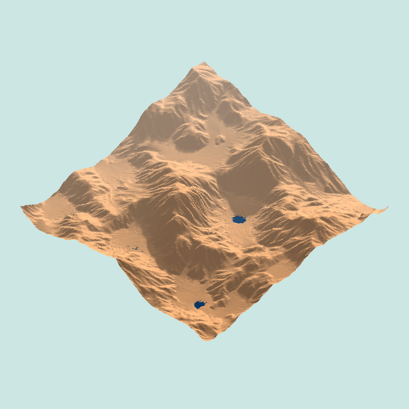
Scree can be modeled explicitly as its own “layer” of sediment, with different friction and solubility / porosity properties than rock. 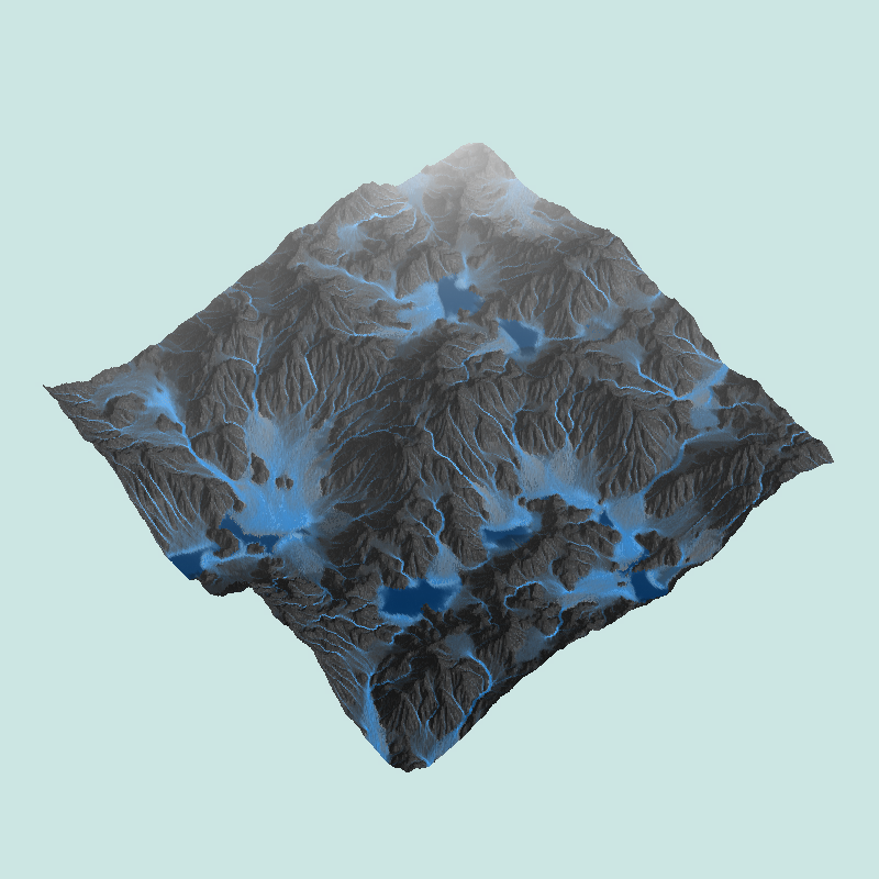
The visible scree in these images is therefore an explicit layer with a defined thickness, a necessary feature for modeling e.g. landslides.
The Layer Map
Note: My singe-header C++ implementation of the layer map can be found on Github here. Note that there are some adjustments made which are explained in subsequent sections.
The simplest data-structure for modeling a height-map is a 2D array of floating point values:
#define DIMX 256
#define DIMY 256

double heightmap[DIMX*DIMY];
To then model multiple layers, a naive approach would be to simply have a fixed number of K “stacked” height-maps. Each height-map stores the extent of the layer at each position, resembling a layer-based run-length encoding.
#define DIMX 256
#define DIMY 256

double heightmap0[DIMX*DIMY]; // Bottom Layer
double heightmap1[DIMX*DIMY];
double heightmap2[DIMX*DIMY];
// ...
double heightmapK[DIMX*DIMY]; // Final, K-th Layer
Note: This would be similar to the concepts used in Simple Hydrology and Simple Wind Erosion, where there is a “ground” heightmap and a “pool” / “sediment” heightmap respectively. This implies a strict, predetermined layer order.
This approach has a number of obvious drawbacks. Storing only the height in each layer implies that the order of layers, with their own soil types and properties, is predetermined.
To overcome this issue, each height-map could instead store a struct which carries additional properties, e.g. the soil type.
// Layer section struct

using SurfType = size_t;

struct sec {
  float h = 0.0f;     //Height
  SurfType type = 0;  //Soil Type Index
};

#define DIMX 256
#define DIMY 256

sec heightmap0[DIMX*DIMY];
sec heightmap1[DIMX*DIMY];
sec heightmap2[DIMX*DIMY];
//...
sec heightmapK[DIMX*DIMY];
Note: The soil type index can be used to derive other properties relevant for erosion processes, such as solubility, friction, color, suspendability, abrasiveness, etc. This is explained below.
While this allows for arbitrary soil types in arbitrary orders with arbitrary layer heights, it is still memory inefficient and limited by a fixed maximum number of layers. A specific location in the domain might have fewer than K layers, while another might have far more.
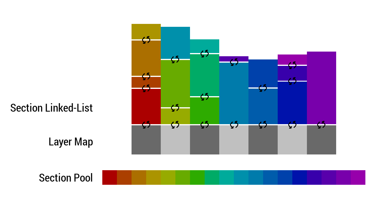
This final issue is overcome by abandoning the fixed number of stacked layer arrays and instead allowing for an arbitrary number of sections at each location in the form of a double linked-list. This final data structure is the layer map.
The Layer Section
The layer section is the main component of the layer map, representing the run-length encoded linked-list element.
using SurfType = size_t;

struct sec {

sec* next = NULL;     //Section Above
sec* prev = NULL;     //Section Below

SurfType type = 0;    //Type of Surface Element
double size = 0.0f;   //Run-Length of Element
double floor = 0.0f;  //Cumulative Height at Bottom

sec(){}
sec(double s, SurfType t){
  size = s;
  type = t;
}

void reset(){
  next = NULL;
  prev = NULL;
  type = 0;
  size = 0.0f;
  floor = 0.0f;
}

};
For traversal, each section contains a pointer to the previous and next sections. For efficient computation of the height, the section also stores its size and the height of its “floor”.
The layer map finally stores a 2D array of section pointers representing the “bottom sections” / “starting points” of the double-linked lists in each location.
// Layer Map

sec** dat = NULL;                        //Raw 2D Data Grid
Layer Section Pooling
As the layer map stores pointers to soil sections, altering the terrain dynamically theoretically requires a lot of memory allocation and de-allocation. It is therefore efficient and convenient to provide a section pool to the layer map.
The section pool is a simple fixed size memory pool which uses a queue to store available section pointers.
class secpool {
public:

int size;               //Number of Total Elements
sec* start = NULL;      //Point to Start of Pool
deque<sec*> free;       //Queue of Free Elements

secpool(){}             //Construct
secpool(const int N){   //Construct with Size
  reserve(N);
}
~secpool(){
  free.clear();
  delete[] start;
}

//Create the Memory Pool
void reserve(const int N){
  start = new sec[N];
  for(int i = 0; i < N; i++)
    free.push_front(start+i);
  size = N;
}

//Retrieve Element, Construct in Place
template<typename... Args>
sec* get(Args && ...args){

  if(free.empty()){
    cout<<"Memory Pool Out-Of-Elements"<<endl;
    return NULL;
  }

  sec* E = free.back();
  try{ new (E)sec(forward<Args>(args)...); }
  catch(...) { throw; }
  free.pop_back();
  return E;

}

//Return Element
void unget(sec* E){
  if(E == NULL)
    return;
  E->reset();
  free.push_front(E);
}

void reset(){
  free.clear();
  for(int i = 0; i < size; i++)
    free.push_front(start+i);
}

};
Layer Map Class and Member Functions
The layer map is thus a 2D array of (memory pooled) run-length encoded soil section doubly-linked lists.
The layer map is wrapped in a simple interface class which stores the section pointer array, section pool and provides a number of useful methods for querying / altering the terrain.
class Layermap {

private:

sec** dat = NULL;                         //Raw Data Grid

public:

ivec2 dim;                                //Size
secpool pool;                             //Data Pool


void initialize(ivec2 _dim){

  dim = _dim;

  //Important so Re-Callable

  pool.reset();

  //Clear Array of Section Pointers

  if(dat != NULL) delete[] dat;
  dat = new sec*[dim.x*dim.y];      //Array of Section Pointers

  for(int i = 0; i < dim.x; i++)
  for(int j = 0; j < dim.y; j++)
    dat[i*dim.y+j] = NULL;

}

//...
Spatial Queries
The layer map spatial queries implement getting the surface height, surface composition and surface normal.
//...

// Queries

sec* top(ivec2 pos){  //Top Element at Position
  return dat[pos.x*dim.y+pos.y];
}

SurfType surface(ivec2 pos){
  if(dat[pos.x*dim.y+pos.y] == NULL) return 0;
  return dat[pos.x*dim.y+pos.y]->type;
}

double height(ivec2 pos){
  if(dat[pos.x*dim.y+pos.y] == NULL) return 0.0;
  return (dat[pos.x*dim.y+pos.y]->floor + dat[pos.x*dim.y+pos.y]->size);
}

vec3 normal(vec2 pos); //this use a cross-product system

//...
Spatial Modifiers
The spatial modification functions either add or remove layers at a location using the section pool.
To add soil at a location, the layer map extends either the run-length encoding or the linked list:
//...

// Add an Element

void add(ivec2 pos, sec* E){

  //Non-Element: Don't Add
  if(E == NULL)
    return;

  //Negative Size Element: Don't Add
  if(E->size <= 0){
    pool.unget(E);
    return;
  }

  //Valid Element, Empty Spot: Set Top Directly
  if(dat[pos.x*dim.y+pos.y] == NULL){
    dat[pos.x*dim.y+pos.y] = E;
    return;
  }

  //Valid Element, Previous Type Identical: Elongate
  if(dat[pos.x*dim.y+pos.y]->type == E->type){
    dat[pos.x*dim.y+pos.y]->size += E->size;
    pool.unget(E);
    return;
  }

  //Add Element
  dat[pos.x*dim.y+pos.y]->next = E;
  E->prev = dat[pos.x*dim.y+pos.y];
  E->floor = height(pos);
  dat[pos.x*dim.y+pos.y] = E;

}

//...
To remove soil at a location, the layer map removes at most the extent of the top section and returns the rest (i.e. non-removed height) if the top section was too small:
double remove(ivec2 pos, double h){

  //No Element to Remove
  if(dat[pos.x*dim.y+pos.y] == NULL)
    return 0.0;

  //Element Needs Removal
  if(dat[pos.x*dim.y+pos.y]->size <= 0.0){
    sec* E = dat[pos.x*dim.y+pos.y];
    dat[pos.x*dim.y+pos.y] = E->prev; //May be NULL
    pool.unget(E);
    return 0.0;
  }

  //No Removal Necessary (Note: Zero Height Elements Removed)
  if(h <= 0.0)
    return 0.0;

  double diff = h - dat[pos.x*dim.y+pos.y]->size;
  dat[pos.x*dim.y+pos.y]->size -= h;

  if(diff >= 0.0){
    sec* E = dat[pos.x*dim.y+pos.y];
    dat[pos.x*dim.y+pos.y] = E->prev; //May be NULL
    pool.unget(E);
    return diff;
  }
  else return 0.0;

}
Note: The return value is important. When removing a certain height of terrain based on the surface composition, the top layer may be too thin, uncovering a new soil layer and thus requiring re-computation of the removal. This is explained in more detail below.
Visualization and Rendering
All visualizations accompanying this article were made by myself using C++ and OpenGL4. To do this I utilize my own TinyEngine, which acts as a small convenient wrapper.
In SoilMachine, I visualize the layer map using the OpenGL AZDO technique “vertex pooling“. A detailed explanation on how vertex pooling works can be found on my blog here.
The layer map class implements a few functions for filling the vertex pool with data for rendering. The exact same technique is also used in the visualization of the current iteration of my Simple Hydrology project.
Note: Vertex pooling was originally written for use with a voxel engine but can be seamlessly applied to terrain rendering.
Multi-Layer Multi-Erosion
The main goal of multi-layer erosion is to simulate multiple erosion processes on maps with non-homogeneous soil composition and distribution.
In this section I would like to explain how the layer map achieves this and allows for simultaneous simulation of hydraulic, thermal and wind erosion.
Additionally, I would like to present how the layer map elegantly handles surface and sub-surface water using layer saturation values, and explain my implementation of pooling (surface and sub-surface, i.e. lakes and ground water in one unified system).
Soil Types and Properties
Different soil types and properties are implemented as a surface parameter struct containing all erosion parameters.
struct SurfParam {

  //General Properties

  string name;
  float density;
  float porosity = 0.0f;
  vec4 color = vec4(0.5, 0.5, 0.5, 1.0);
  vec4 phong = vec4(0.5, 0.8, 0.2, 32);

  //Hydrologyical Parameters

  SurfType transports = 0;    //Surface Type it Transports As
  float solubility = 1.0f;    //Relative Solubility in Water
  float equrate = 1.0f;       //Rate of Reaching Equilibrium
  float friction = 1.0f;      //Surface Friction, Water Particles

  SurfType erodes = 0;        //Surface Type it Erodes To
  float erosionrate = 0.0f;   //Rate of Conversion

  //Cascading Parameters
  SurfType cascades = 0;      //Surface Type it Cascades To
  float maxdiff = 1.0f;       //Maximum Settling Height Difference
  float settling = 0.0f;      //Settling Rate

  //Wind Erosion
  SurfType abrades = 0;       //Surface Type it Cascades To
  float suspension = 0.0f;
  float abrasion = 0.0f;      //Rate at which particle size decreases

};
The set of surface parameters is stored in a global vector, and the indices of different soils are accessible using a map.
vector<SurfParam> soils = {

    { "Air", 0.0f, 1.0f,
      vec4(0.0, 0.2, 0.4, 1.0),
      vec4(0.5, 0.8, 0.2, 32),
      0, 0.0f, 0.0f, 0.0f,
      0, 0.0f,
      0, 0.0f, 0.0f,
      0, 0.0f, 0.0f}

};

map<string, int> soilmap = {

  {"Air", 0}

};
An important assumption made here is that all soils belong to a discrete set of types. Layer map sections do not support mixtures or property mixtures, which would be memory intense and requires more work to solve elegantly.
The Sediment Conversion Graph
One important observation is that as sediment undergoes erosion, its physical properties are often changed.
Massive rock undergoing thermal erosion for instance breaks off into loose boulders, chunks of rock and gravel which has different porosity, solubility and friction.
Particularly in the absence of soil type mixtures, there is no concept of a continuous variation of parameters based on composition changing from one soil type to another.
To model how sediment types can be converted into other sediment types as they are transported, the parameter struct contains references to other sediments by their index. This produces the sediment conversion graph.
Examples of other natural transport and conversion processes which are relevant include compression, petrification, dissolution and crystallization, fracturing, abrasion, etc.
Note: The conversion graph is not implemented explicitly as a graph but implicitly by the references in the parameter struct. The referenced sediment types are accessed in the functions which model the physical conversion processes. A possible alternative to this model is explored at the end of this article.
Run-Time Configuration: .soil File Format
The only type of soil (i.e. “layer class”) which I define by default is air (the non-soil). The utility of storing the surface parameters using a vector and map is that they can be loaded at run-time from a configuration file.
To do this, I provide .soil files, which have a simple mark-up format for defining a set of soil types with parameters and a configuration for the world. This avoids lots of compiling and allow for easy tuning of parameters and initial conditions.
Note: The .soil file also allows to define the set of initial condition layers with simplex noise parameters and rendering parameters for a phong-based lighting model. Default File. I was doing a lot of re-compiling prior to implementing this.
Generalizing Particle-Based Erosion
To simultaneously simulate different erosion processes, I decided to generalize the particle based erosion concept.
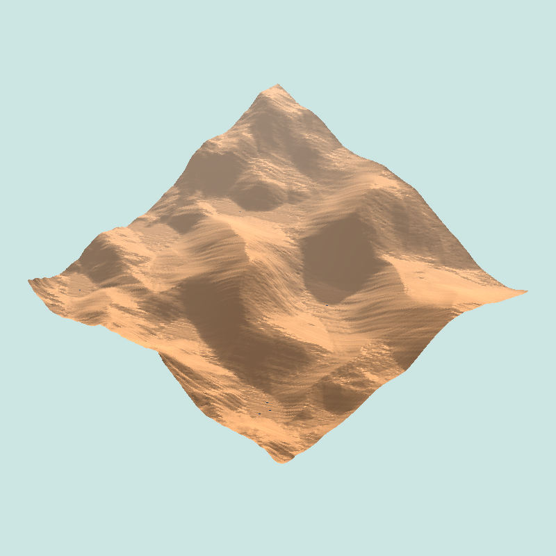
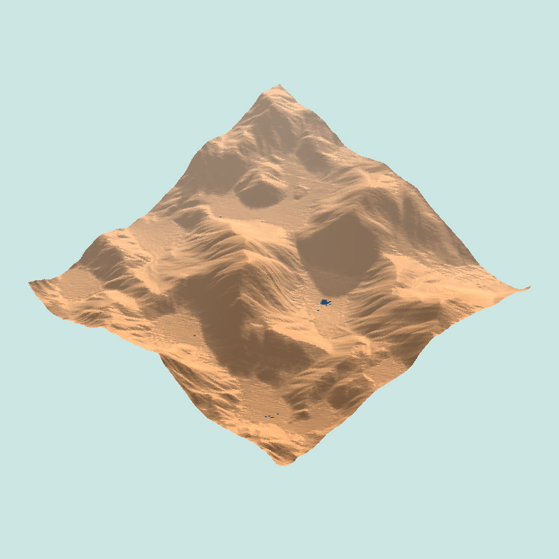
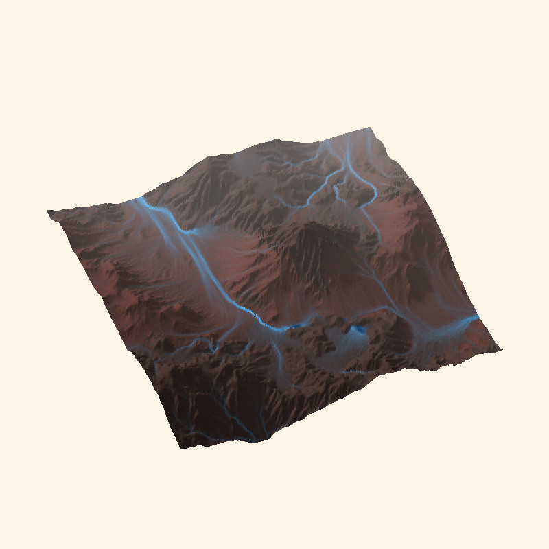
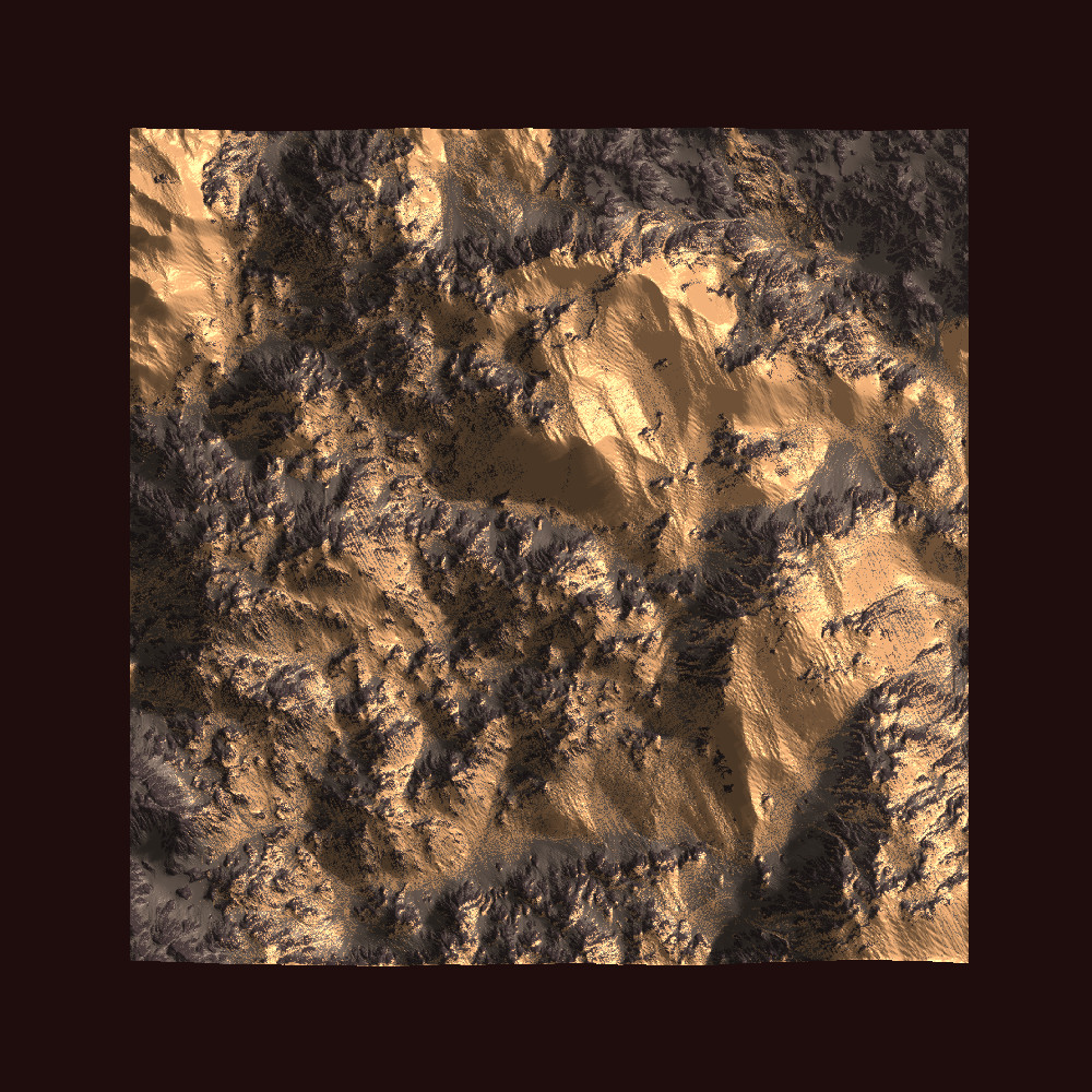
Note: In the images above, you can see the same map eroded three times with different amounts of wind and rain. The soil is a highly erosive sand.
To do this, I decided to implement a particle base class.
The particle base-class stores a position, a speed and whether the particle is alive. The map interaction is defined by two processes: movement and surface interaction.
struct Particle {

  vec2 pos;
  vec2 speed = vec2(0);
  bool isalive = true;

  bool move(Layermap& map);
  bool interact(Layermap& map, Vertexpool<Vertex>& vertexpool);

  static void cascade(vec2 pos, Layermap& map, Vertexpool<Vertex>& vertexpool, int transferloop = 0);

};
Note: To compute the movement, the particle requires the layer map (e.g. surface normals). The same is valid for the interaction, which can also directly update the vertex pool for rendering. Both methods return booleans to indicate completion.
Hydraulic and wind erosion are then implemented as a derived class of the particle base class, described below.
Sediment Cascading
The particle base class implements the static cascade method, which is the process by which sediment or soil at a specific location achieves its talus angle (see scree).
This is a process that can be triggered by a variety of events and is computed based solely off of location and surface composition; hence its implementation as a static method.
Note: I have described in detail the theory and implementation of sediment cascading in my Simple Wind Erosion project.
For multi-layer cascading, some modifications are made. Cascading now uses a height-sorted 8-way neighborhood stored in a temporary vector for simplicity (and sorting).
  static void Partice::cascade(vec2 pos, Layermap& map, Vertexpool<Vertex>& vertexpool, int transferloop = 0){

    ivec2 ipos = round(pos);

    // All Possible Neighbors

    const vector<ivec2> n = {
      ivec2(-1, -1),
      ivec2(-1,  0),
      ivec2(-1,  1),
      ivec2( 0, -1),
      ivec2( 0,  1),
      ivec2( 1, -1),
      ivec2( 1,  0),
      ivec2( 1,  1)
    };

    //No Out-Of-Bounds

    vector<ivec2> sn;
    for(auto& nn: n){
      ivec2 npos = ipos + nn;
      if(npos.x >= map.dim.x || npos.y >= map.dim.y
         || npos.x < 0 || npos.y < 0) continue;
      sn.push_back(npos);
    }

    // Sort by Highest First (Soil is Moved Down After All)

    sort(sn.begin(), sn.end(), [&](const ivec2& a, const ivec2& b){
      return map.height(a) > map.height(b);
    });

    // ...
The cascade iterates over eligible neighbors and retrieves the surface parameters of the higher (i.e.: falling) location using the layer map and global parameter vector.
Finally, the layer map is modified using the built-in methods.
    for(auto& npos: sn){

      //Full Height-Different Between Positions!
      float diff = (map.height(ipos) - map.height(npos))*(float)SCALE/80.0f;

      if(diff == 0)   //No Height Difference
        continue;

      ivec2 tpos = (diff > 0) ? ipos : npos;
      ivec2 bpos = (diff > 0) ? npos : ipos;

      SurfType type = map.surface(tpos);
      SurfParam param = soils[type];

      //The Amount of Excess Difference!
      float excess = abs(diff) - param.maxdiff;
      if(excess <= 0)  //No Excess
        continue;

      //Actual Amount Transferred
      float transfer = param.settling * excess / 2.0f;

      bool recascade = false;

      if(transfer > map.top(tpos)->size)
        transfer = map.top(tpos)->size;

      if(map.remove(tpos, transfer) != 0)
        recascade = true;
      map.add(bpos, map.pool.get(transfer, param.cascades));
      map.update(tpos, vertexpool);
      map.update(bpos, vertexpool);

      if(recascade && transferloop > 0)
        cascade(npos, map, vertexpool, --transferloop);

    }

  }
Re-cascading is triggered if the return value of remove is non-zero. This implies that the slope is unstable but the surface section was too shallow. The cascading process is repeated at the same location with the parameters of the newly exposed surface section.
Note: Re-cascading is recursive until the depth transferloop.
Water and Wind Particle Derived Classes
struct WaterParticle : public Particle;
struct WindParticle : public Particle;
The wind and water particle classes implement the move and interact methods of the particle base class and derive the surface parameters using the layer map and surface parameter map. Each particle additionally tracks the soil type which it contains in order to place soil on the map.
Note: More detailed implementation details for these derived classes can be found in my previous projects Simple Hydrology and Simple Wind Erosion. Some modifications have of course been made in this project.
To execute the erosion cycles every frame, we simply spawn a particle on the map (using its own constructor) and allow it to move and interact until it declares itself dead or finished.
if(dowatercycles)
for(int i = 0; i < NWATER; i++){

    WaterParticle particle(map);

    while(particle.move(map, vertexpool) && particle.interact(map, vertexpool));

}

if(dowindcycles)
for(int i = 0; i < NWIND; i++){

    WindParticle particle(map);

    while(particle.move(map, vertexpool) && particle.interact(map, vertexpool));

}
Layer Saturation and Water Model
The layer map offers an intuitive and direct manner to model water on (and in) terrain by using a concept of saturation. In this section, I would like to present this concept in detail.
Each soil type has a parameter porosity which determines a layers porous volume (i.e. how much water it can absorb). An air layer for instance has porosity 1.
We give each layer section an additional floating point value saturation, which uses a value between 0 and 1 to define how much of the porous volume is filled with water.
struct sec {
//...

double saturation = 0.0f;         //Saturation with Water

//...
};
Sub-surface layers therefore directly know their water content for modeling ground water, while saturated air layers are used to model surface water.
Water Placement: Flooding
The water particle implements a flooding method which is called when its movement and interaction terminate:
if(dowatercycles)
for(int i = 0; i < NWATER; i++){

    WaterParticle particle(map);

    while(true){
        while(particle.move(map, vertexpool) && particle.interact(map, vertexpool));
	if(!particle.flood(map, vertexpool))
	    break;
    }

}
This method attempts to place any remaining particle sediment and water volume on the map, after which it terminates the particle. In contrast to my previous flooding implementation, water is now placed at a single location!
bool WaterParticle::flood(Layermap& map, Vertexpool<Vertex>& vertexpool){

    if(volume < minvol || spill-- <= 0)
      return false;

    ipos = pos;

    // Add Remaining Soil, Move the Soil

    map.add(ipos, map.pool.get(sediment*soils[contains].equrate, contains));
    Particle::cascade(pos, map, vertexpool, 0);

    // Add Remaining Water Volume, Move the Water

    map.add(ipos, map.pool.get(volume*volumeFactor, soilmap["Air"]));
    seep(ipos, map, vertexpool);
    WaterParticle::cascade(ipos, map, vertexpool, spill);

    // Update Map, Terminate

    map.update(ipos, vertexpool);
    return false;

  }
Note that flooding water is always added at the surface as a saturated layer of air. The water particle finally implements two methods for water movement: cascade and seep.
Water Movement: Cascade
The water particle implements the static cascade method which acts only on surface water (i.e. saturated air layers).
In full analogy to sediment cascading, the water cascade method is a local cellular automaton which equilibriates the height difference to zero, implying a friction-less medium.
Finally, when cascading occurs towards a position which is below the floor of the saturated air layer, the volume of the layer is converted back to a descending water particle.
Note: This is very similar to cellular automata style water movement found in many hydrology research papers.
Water Movement: Seeping
The water particle static seep method attempts to move water between neighboring layer sections by their porosity.
Ideally, based on relative water pressure between sections, the direction of water movement can be computed. The porosity values of different sections can then be used to compute the seepage rate at which saturation is transferred.
  static void seep(vec2 pos, Layermap& map, Vertexpool<Vertex>& vertexpool){

    ivec2 ipos = pos;

    sec* top = map.top(ipos);
    double pressure = 0.0f;            //Pressure Increases Moving Down
    if(top == NULL) return;

    // Move Downwards

    while(top != NULL && top->prev != NULL){

      sec* prev = top->prev;

      SurfParam param = soils[top->type];
      SurfParam nparam = soils[prev->type];

      // Water Volume Top Layer
      double vol = top->size*top->saturation*param.porosity;

      //Volume Bottom Layer
      double nvol = prev->size*prev->saturation*nparam.porosity;

      //Empty Volume Bottom Layer
      double nevol = prev->size*(1.0 - prev->saturation)*nparam.porosity;

      // Constant
      double seepage = 1.0;

      //Transferred Volume is the Smaller Amount!
      double transfer = (vol < nevol) ? vol : nevol;

      if(transfer > 0){

        // Remove from Top Layer
        if(top->type == soilmap["Air"])
          double diff = map.remove(ipos, seepage*transfer);
        else
          top->saturation -= (seepage*transfer) / (top->size*param.porosity);

        prev->saturation += (seepage*transfer) / (prev->size*nparam.porosity);

      }

      top = prev;

    }

    map.update(ipos, vertexpool);

  }
Note: The seep method is currently only implemented for downward water movement at a constant seepage rate. See the results and discussion and next steps for more information.
Layer Map Implementation Detail: Adding Water
The layer map add function is modified to take into account placement of layer sections on top of air layers. The air layer remains on top so sediment “falls below” the water layer.
void Layermap::add(ivec2 pos, sec* E){

  //... already handled adding water to water ...

  //Add something that is not water to water
  //Basically: A position Swap

  if(dat[pos.x*dim.y+pos.y]->type == soilmap["Air"]){

    //Remove Top Element (Water)
    sec* top = dat[pos.x*dim.y+pos.y];
    dat[pos.x*dim.y+pos.y] = top->prev;

    //Add this Element
    add(pos, E);

    //Add Water Back In
    add(pos, top);

    //Finished
    return;

  }

//...

}
Results and Discussion
The Layer Map
I believe that the layer map works quite well.
The layer map is easily voxelized after the fact, which I did for visualization in yet another project of mine.
Section pool cache coherency doesn’t appear to be an issue during simulation, but might be a consideration if the data should be stored. The section pool could be written to file with a sorting pass such that it is ordered by the pointers, instead of by the time of allocation.
The rate of section pool filling depends on the number of soil types used, as there is less potential for layer merging and more potential for thin slivers of layers to stack.
An important aspect that I have not been able to wrap my head around is layer swapping and “compression”.
Sediments compressing under pressure represents a link in the sediment conversion graph, but how does one compress multiple layers together? The layers could be “sorted” or “swapped” somehow, but by what rules? This is an issue of modeling discrete sediment classes instead of mixtures.
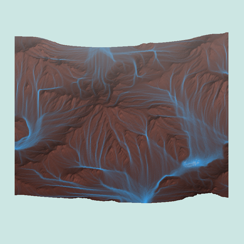
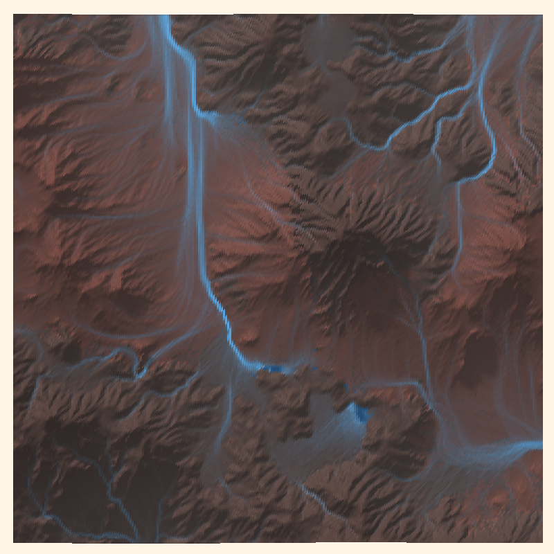
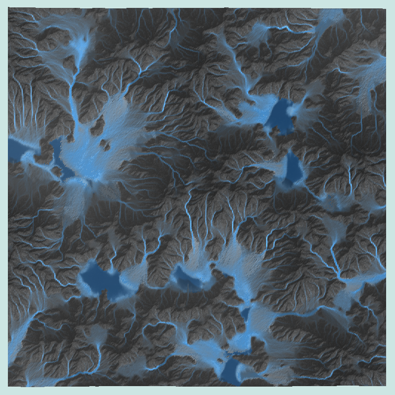
A landscape with very erosive soil undergoing hydraulic erosion. 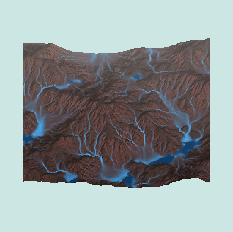
The same landscape undergoing hydraulic erosion, but this time with a thin layer of erosion resistant cap rock. Note the formation of pooling on top of the non absorbent / porous layer.
Improved Water Model
Previously, I was using a form of rapid-flood spilling method, which computes a global solution to the water placement and requires many flood fill operations and height queries. These are both computationally expensive, representing the main bottleneck of my previous system.
Note: I tried improving efficiency by iterating only over the sorted boundary and storing state in intelligent structs, but this quickly became complex with yet insufficient performance.
With the cascading-based, local cellular automaton, the process of water surface equilibriation is deferred over many frames, vastly improving performance and giving the surface water an explicit movement speed.
Additionally, it easily overcomes the buggiest aspect of the rapid flood spilling, which was degenerate height-map cases and drainage points.
Now, it just works.
Multi-Layer Multi-Erosion
I am also quite pleased with the ability to have multiple erosion processes operating simultaneously on the same map with different soil properties at different points. Surprisingly, this didn’t give me much of a hard time.
Sand on a hard rock which erodes into a more loose rock (3 soil types). 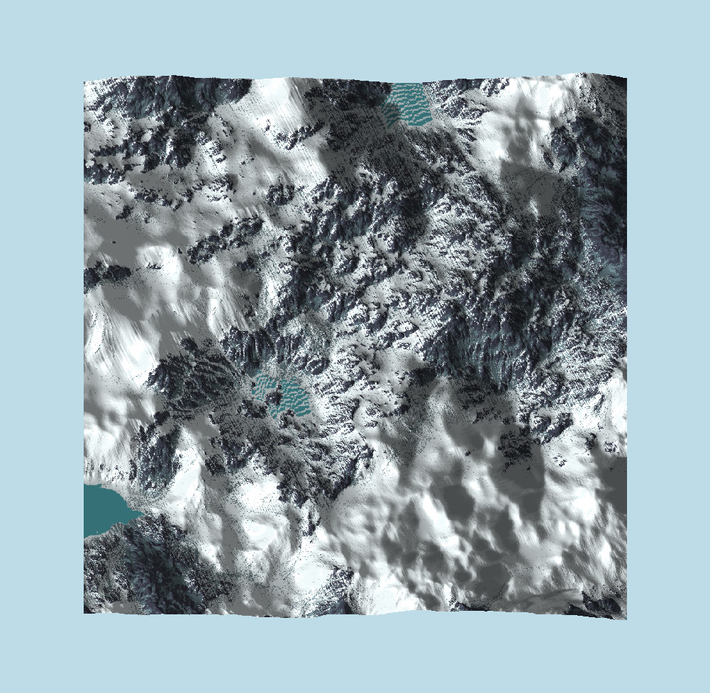
Snow blowing over a hard rocky landscape.
This works well and the differences in soil properties become all the more striking when you can see them on the same map at the same time. Also you can do fun things like snow blowing over landscapes or dump sand on mountains.
Future Directions
The layer map concept represents a starting point for a unified multi-layer, multi-erosion terrain generator and opens up many interesting avenues for expansion that I would like to explore in the future.
Side-Ways Spatial Queries
Implementing sideways spatial queries is an essential step towards reaching the full potential of the layer map.
Erosion processes don’t always remain “on the surface”, but also require interaction with exposed sub-surface layers. This is apparent in e.g. coastal erosion or overhangs (i.e. eroding away from underneath).
Additionally, it is necessary to model sideways sub-surface seepage for groundwater flow and thus cave generation.
Note that a major hurdle that still needs to be overcome is efficient meshing and rendering of caves and overhangs, as the vertex pool currently still only renders surface data.
Note: A practical implementation of sideways spatial queries might rely on C++ style iterators. Landslides and avalanches are also related and require sideways spatial queries!
Erosion Particle Spawn Distributions
One aspect which I have been working on for a long time is finding appropriate distributions for spawning particles.
My first attempt was with my 2D procedural weather system (cellular automaton), which became a 2.5D finite-volume based weather simulation MicroClimate, and is currently evolving into a full 3D Lattice-Boltzmann based simulation.
This is still a work in progress, and while mostly complete, remains on my write-up backlog.
Vegetation Particles
A very natural extension of the generalized particle system and SoilMachine would be vegetation particles. With the new availability of ground water level and depth, a realistic modeling of vegetation becomes possible.
A simple model would be to have a set of vegetation classes (i.e. species) with properties dictating e.g. root depth and spread, water requirements, “canopy” size, sunlight requirements and reproductive rates.
Allowing the particles to multiply and compete (by de-spawn rates when requirements are insufficiently satisfied), they should then naturally converge to a stable distribution with strong coupling to the terrain.
Additionally, the modification of sediment layers by plants and the creation of biomass layers (e.g. peat and thus coal) is a vital aspect of the geological cycle that can be easily modeled using the de-spawning of vegetation particles.
Efficiency Improvements
The main drawback of the particle-based erosion simulation is its sequential nature. This becomes particularly apparent when eroding noise-based terrain, which exhibits many local minima when used as an initial condition, in which particles waste computation cycles.
Applying a level-of-detail based erosion simulation could help to eliminate local minima at small scales efficiently and allow for parallel simulation at various scales (see wavelets).
Additionally, splitting the map into multiple sub-regions and merging these intelligently allows for further parallelization. The new particle base class then provides a convenient interface for this parallelization.
Note that a Morton ordering of the layer map root pointers (i.e.: quad-tree) would not only allow for easy multi-scale simulation using an index stride, but also for easy splitting of the map into equally sized sub-regions.
This concept is in its infancy and warrants its own project, but I also already have a rough code outline written for this.
Note: These ideas have the potential to introduce boundary artifacts and non-deterministic aspects, so these trade-offs need to be weighed and balanced by good concepts.
Mixtures and Multiple Fluids
The key assumption of the layer map is its discrete set of sediment classes. This also applies to fluids, as each layer section only stores a single saturation value without a type.
This is a strong assumption which breaks with simple ideas such as “loose rocks in a pile of sand”. It could potentially also be desirable to model multiple fluids or fluid phases separately, such is brine or oil.
A future implementation of “mixed layers” would require an intelligent extension to the layer section structure as well as consideration of layer property mixing rules.
Note that the section pool works best as a fixed-size memory pool. One way to keep this requirement and allow for mixtures is for layer sections to store pointers to “virtual layers”, which together comprise the layer mixture. This would also work for fluids.
Final Words
This post is merely one of a long backlog of half-written projects which I hope to spend more time on soon. Of course I always say that and it never pans out that way.
Still I had a great time building this and this (in particular SoilMachine) really represents the culmination of a few years of work on simulated geomorphology and particle-based erosion. Nevertheless, the more I work on it, the more I realize I have barely scratched the surface.
Feel free to reach out if you have questions about anything in this article and thank you for reading until the end!