Note: The full source code for this system can be found [here].
Once again I find myself working on a procedural system (discretizing my world generation systems into voxels) and limited by the power of the data visualization (my engine).
I decided to take another general look at voxel engines to see if I could come up with any improvements now that I have some more experience in graphics programming. In particular, I wanted to look at optimization techniques for rendering voxel data while focusing mainly on vertex memory management and driver overhead reduction.
Note: My previous voxel engine Homebrew Voxel Engine was not sufficiently performant and generally required a major refactor of the rendering code due to feature creep.
I call the system that I came up with a Vertex Pool, and it combines the power of modern OpenGL with concepts from memory pooling to provide extremely fast voxel meshing / re-meshing and extended occlusion queries which are normally not possible using typical rendering approaches, offering unique new avenues for optimization.
Much of this system was inspired by the “Approaching Zero-Driver Overhead” talk given at GDC which I finally had the pleasure of watching. I highly recommend it.
In the following article, I would like to showcase this system and its advantages with an extensive set of benchmarks. There are many aspects to discuss, so this could be long. I hope you like memory management.
Finally, I will showcase how this system can be used to seamlessly visualize large voxel worlds from memory.
The system is capable of rendering upwards of 50×50 randomized 4-color (very bad case, more info later) chunks of volume 32x32x32 at over 30 FPS from the CPU.
Compared to a naive implementation with a VAO / VBO per chunk, it improves frames times by up to 40% and meshing times by up to 25% due to lower driver overhead and better garbage collection for an identical geometry. Additionally, it bypasses all memory management difficulties associated with a single merged VAO / VBO system.
Note: The system is theoretically applicable to any kind of vertex data and not just voxel based systems. A few additional nice optimizations exist for voxels and they are a good example!
Voxel Data Rendering Systems
Note: I make the key assumption that voxel occupation data is stored data in CPU memory and not “computable”, e.g. given by a noise function. Alternative engine designs exist and are more performant when voxel data is computable (i.e. offload everything to GPU). I assume voxels are represented by cubes.
A number of possible techniques come to mind for rendering stored voxel data (independent of storage):
- Compact Cube Meshes with Instancing
- Point Voxels with Geometry Shader Cubing
- Chunking + Chunk Meshing
I will briefly discuss these techniques below for context.
Instancing and Geometry Shaders
Instancing is a well known OpenGL technique for rendering large amounts of identical data. For voxels, the idea is to render the same cube model multiple times under different transformations. Since all voxels are axis-aligned, it is initially sufficient to pass 3 coordinates per voxel to the vertex shader to specify the instance position.
Geometry shaders is a GPU-based method to generate render primitives from data. The geometry shader technique might take a 3 coordinate position per voxel and expand it into a set of primitives representing a cube for rendering.
Note: Geometry shaders are implemented in software which is a significant drawback out of the gate.
The key idea behind these techniques is to minimize the amount of data being streamed to the GPU, but in their naive form they suffer from a large amount of fragment waste due to non-consideration of voxel neighbor information.
Passing per-neighbor information is possible for both of these techniques: face visibility can be stored in a single byte (6 Faces, Visible or Not: 2^6 = 64).
The geometry shader would use this information to not emit primitives where they aren’t required, while the instanced rendering system would need to draw separate models for each neighbor connection possibility.
Naively, the instanced renderer requires 64 instanced draw calls, but can be reduced to 8 by streaming an additional byte of orientation data.
Each instanced draw call now requires its own buffer with position and orientation information. Consider the effect of changing of a single voxel: In the worst case (all neighbors in different instance groups), the 6 neighbors now require the resizing and re-uploading of 6 of these instanced draw buffers, increasing driver overhead.
Both of these techniques are known to suffer from a lack of scalability and other performance issues which I won’t discuss further.
Note: At some point, our memory management is totally lost in the sauce while suffering from additional driver overhead. There are other considerations that I won’t go into here.
Chunking and Chunk Meshing
Note: This is the most common technique found online and is also the technique I used in my Homebrew Voxel Engine with “greedy meshing”. In the remaining article, I will assume a system of this type as the baseline for comparison.
Instead of observing data on a per-cube basis, it is possible to mesh the totality of the voxel data on the CPU, which is then rendered using one or more regular indexed draw calls.
In contrast, both the geometry shader and instancing methods fail to address the simple fact that multiple cube’s surfaces can be combined. With a 16^3 volume of identical cubes, they would execute 16^3 instanced draws or geometry shader cube expansions, when a mesh would actually only consist of 6 quads.
The consideration of all voxel data simultaneously when generating the mesh reduces the total number of vertices drawn and eliminates all fragment waste generated due to (intrinsically) non-visible surfaces. Typical algorithms to produce such a mesh are Greedy- and Monotone Meshing
Finally, the idea behind “chunking” is to subdivide the world voxel data into sections, so that the world can be edited / loaded / unloaded and meshed based on location (and sub-meshes stored in separated memory are easier to modify).
This approach generally yields high performance but starts to suffer from large driver overhead when rendering large numbers of separate chunks, as a single draw call is usually issued for every chunk mesh after changing the driver state.
During testing I found that combining multiple chunks into a single VAO + VBO system can lead to significant decreases in frame times, indicating a large amount of state-change driver overhead when using non-merged chunk meshes.
Note: This is also what they will tell you in the “Approaching Zero Driver Overhead” talk at GDC. Merge your VAOs / VBOs.
The problem with this is that with a merged VBO, it becomes very tedious to update sub-regions (i.e. individual sub-meshes) without having to resize and re-upload the entire VBO (all chunks) to the GPU, which is not required when each chunk has its own mesh memory (VAO / VBO).
Note: Instead of slicing out sub-mesh data and re-uploading the entire buffer, you could “invalidate” it, update only a section of the buffer and issue two draw calls on the split buffer, but eventually we will be issuing draw calls for every sub-mesh in the merged VBO. This overhead is precisely what we tried to avoid. Once again, we find ourselves lost in the memory sauce.
This represents my core problem with existing techniques:
There is an intrinsic trade-off between simplicity of mesh memory management and driver overhead required for state changes and issuing draw calls.
This is what the vertex pool renderer attempts to overcome.
Vertex Pool Rendering
The core idea behind the Vertex Pool is to utilize a persistently mapped VBO as a memory pool containing interleaved vertex data. The vertex pool manages a set of fixed-size vertex buckets to which it provides access when new mesh storage is requested. Finally, each occupied bucket is associated with an entry in an indirect draw call buffer utilized together with glMultiDrawElementsIndirect.
Note: None of these ideas are new. I just haven’t seen them combined in this way and discussed anywhere online.
Using this structure we can simultaneously reduce driver overhead, essentially merging many sub-meshes, while keeping memory management simple.
In combination, these concepts perform better than regular chunk meshing in terms of garbage collection, getting data to the GPU and CPU based occlusion queries. This system will be described in detail below with code samples in C++.
Note: The entire code described below can be found in a single file [here] with about 350 LOC. It is a working implementation of persistently mapped buffers with interleaved vertex data, fast greedy meshing and glMultiDrawElementsIndirect. I will not go into too much detail about the individual techniques, but will link relevant information and sources whenever possible.
Interleaved Vertex Data Format
It is not uncommon to have multiple VBOs store the data of individual shader attributes. This means there can exist e.g. a VBO for position, normal and texture data.
Alternatively we can specify an “interleaved format” so that all shader attributes for a vertex are stored in a single VBO. This has a number of potential benefits, particularly for memory pooling vertices.
An example implementation of a vertex data-structure with a built-in formatting function for a VBO could be:
using namespace glm;

struct Vertex {

  float position[3];
  float normal[3];
  float color[4];

  Vertex(vec3 p, vec3 n, vec3 c){

    position[0] = p.x;
    position[1] = p.y;
    position[2] = p.z;
    normal[0] = n.x;
    normal[1] = n.y;
    normal[2] = n.z;
    color[0] = c.x;
    color[1] = c.y;
    color[2] = c.z;
    color[3] = 1.0;

  }

  static void format(int vbo){

    glEnableVertexAttribArray(0);
    glEnableVertexAttribArray(1);
    glEnableVertexAttribArray(2);

    glVertexAttribFormat(0, 3, GL_FLOAT, GL_FALSE, 0);
    glVertexAttribFormat(1, 3, GL_FLOAT, GL_FALSE, 0);
    glVertexAttribFormat(2, 4, GL_FLOAT, GL_FALSE, 0);

    glVertexBindingDivisor(0, 0);
    glVertexBindingDivisor(1, 0);
    glVertexBindingDivisor(2, 0);

    glVertexAttribBinding(0, 0);
    glVertexAttribBinding(1, 1);
    glVertexAttribBinding(2, 2);

    glBindVertexBuffer(0, vbo, offsetof(Vertex, position), sizeof(Vertex));
    glBindVertexBuffer(1, vbo, offsetof(Vertex, normal), sizeof(Vertex));
    glBindVertexBuffer(2, vbo, offsetof(Vertex, color), sizeof(Vertex));

  }

};
Note: This is the data structure I use in my implementation, but it is easily modifiable to have alternative per-vertex properties.
To initialize the VAO and interleaved VBO of our vertex pool, we simply call the format function upon construction. Note that the vertex pool class is templated by the Vertex struct.
template<typename T>
class Vertexpool {
private:

//...

GLuint vao;     //Vertex Array Object
GLuint vbo;     //Vertex Buffer Object

public:

//Default Constructor (Handles VBO Interleaving)
Vertexpool(){

  glGenVertexArrays(1, &vao);
  glBindVertexArray(vao);
  glGenBuffers(1, &vbo);
  T::format(vbo);

}

//...

}
The corresponding shader attributes are thus correctly extracted from the VBO containing a contiguous set of Vertex structs.
Persistent Mapping and Vertex Pool
Persistent VBO mapping is an AZDO technique that lets you allocate a fixed size buffer and keep it mapped, yielding a pointer to which data can be written directly from the CPU.
We can use the mapped buffer as a memory pool by dividing it into a set of N fixed size buckets of size K. We finally store the pointers to the available buckets in a queue:
///... in Vertexpool class

public:

//Constructor with Bucket Size and Number
Vertexpool(int k, int n):Vertexpool(){
  reserve(k, n);
}

private:

size_t K = 0;    //Number of Vertices per Bucket
size_t N = 0;    //Number of Maximum Buckets

T* start;        //Start of Persistent Mapped VBO
deque<T*> free;  //Queue of Free Bucket Pointers

//Function to Map the Vertex Memory Pool / Buffer
void reserve(const int k, const int n){

  K = k; N = n;
  const GLbitfield flag = GL_MAP_WRITE_BIT | GL_MAP_PERSISTENT_BIT | GL_MAP_COHERENT_BIT;

  glBindBuffer(GL_ARRAY_BUFFER, vbo);
  glBufferStorage(GL_ARRAY_BUFFER, N*K*sizeof(T), NULL, flag);
  start = (T*)glMapBufferRange( GL_ARRAY_BUFFER, 0, N*K*sizeof(T), flag );

  for(int i = 0; i < N; i++) //Initialize Buckets
    free.push_front(start+i*K);

}

//...
Note: Our reason for using a queue is so that we can quickly insert in the front and retrieve from the back. This FIFO system means that if we allocate more buckets than we actually use, then the next requested bucket will always point to the region of memory which was cleared the longest time ago, meaning that we avoid double buffering / synchronization problems.
Our goal is to associate every occupied vertex bucket with its own draw call for rendering and memory management.
Multidraw-Indirect and Rendering
glMultiDrawElementsIndirect is a technique which allows for offloading the issuing of draw calls to the GPU using an indirect draw call buffer, which contains a contiguous set of “indirect draw call structs” (DAIC). A DAIC struct has a set of members determining all required draw call parameters.
Note: I will refer to a draw call struct as DAIC (“Draw Elements Arrays Indirect Command”) from here on. Slight misnomer.
We define the DAIC struct with a default constructor:
struct DAIC {

  DAIC(){}
  DAIC(uint c, uint iC, uint s, uint bV, uint* i){

    //Base Properties
    cnt = c; instCnt = iC; start = s; baseVert = bV; baseInst = 0;

    //Additional Properties
    index = i;

  }

  //Base Properties
  uint cnt;       //Total Number of Indices to Draw
  uint instCnt;   //Total Number of Instances
  uint start;     //First Index to Draw (Start pos in index buffer)
  uint baseVert;  //First Vertex to Draw (i.e. start pos in VBO)
  uint baseInst;  //Not quite sure... not important for me lol (I think)

  //Additional Properties (at end!)
  uint* index;

};
A DAIC specifies the starting location and draw length in the index buffer, as well as the start position in the vertex buffer.
It is also possible to append properties to a DAIC struct. Most importantly, I give each DAIC an additional pointer to an unsigned int storing that particular DAIC’s index in the indirect draw command buffer. This is explained later!
With a contiguous memory data structure containing DAIC structs, we can easily upload the draw calls to the GPU. Additionally, because we are using indexed draw calls, we create an index buffer and upload the indices to the GPU:
//... in Vertexpool class

private:

GLuint ebo;     //Element Array Buffer Object
GLuint indbo;   //Indirect Draw Command Buffer Object

Renderpool(){

  //...

  glGenBuffers(1, &ebo);
  glGenBuffers(1, &indbo);

  //...

}

vector<DAIC> indirect;  //Indirect Drawing Commands (Contiguous)
vector<GLuint> indices;

//Upload the Draw Commands to GPU
void update(){

  glBindBuffer(GL_DRAW_INDIRECT_BUFFER, indbo);
  glBufferData(GL_DRAW_INDIRECT_BUFFER, indirect.size()*sizeof(DAIC), &indirect[0], GL_DYNAMIC_DRAW);

}

void index(){

  //... fill index vector (explained later)

  glBindBuffer(GL_ELEMENT_ARRAY_BUFFER, ebo);
  glBufferData(GL_ELEMENT_ARRAY_BUFFER, indices.size()*sizeof(GLuint), &indices[0], GL_STATIC_DRAW);

}

//...
Finally, if all buffers are filled and uploaded the draw calls are issued by binding all the relevant buffers and issuing the multi-indirect function call (without sync checking here):
//...

void render(const GLenum mode = GL_TRIANGLES, size_t first = 0, size_t length = 0){

  //... bounds checking, modifying length, etc.

  glBindVertexArray(vao);
  glBindBuffer(GL_ELEMENT_ARRAY_BUFFER, ebo);
  glBindBuffer(GL_DRAW_INDIRECT_BUFFER, indbo);

  glMultiDrawElementsIndirect(mode, GL_UNSIGNED_INT, (void*)(first*(sizeof(DAIC))), length, sizeof(DAIC)); //here

}

//...
Note that the parameters passed to the draw call here specifically allow the DAIC struct to have extra members.
The remaining task is to fill the indirect draw command buffer, vertex buffer and index buffer intelligently.
Note: Strictly speaking we would require a GPU synchronization lock placed around the draw call to guarantee that all writes to the persistently bound VBO are completed before continuing, but using our queued vertex pool we essentially already apply a form of multi-buffering (double / triple). I couldn’t get the locks to work consistently so I left them out – if you can fix this feel free to contact me.
Contiguous Non-Strict Ordered Memory
Note: This is a small (but important!) section explaining why each DAIC stores a pointer to its index in the DAIC buffer.
In the DAIC buffer, we have a set of draw calls which each correspond to a vertex pool bucket with mesh data. To keep track of the occupied buckets of the vertex pool, it suffices to keep track of the DAIC associated with a sub-mesh in the vertex pool. So how do we do store a reference to a DAIC?
Two possible methods come to mind: Storing an index of the DAIC struct or a pointer to the DAIC struct.
Note that the DAIC buffer must exist in contiguous memory to be passed to the GPU, but that this also imposes an order.
This causes a number of inconveniences:
- Index and pointer references to draw calls are both invalidated if the strict order is not kept (i.e. erased elements, sorting)
- Erasing a draw call from the vector in strict ordering can be an expensive operation for large vectors.
- Pointer references can additionally be invalidated if the vector is reallocated for some reason
Note: We can’t use a data structure like an std::deque which never invalidates pointers because we need the data contiguity.
This strict ordering in contiguous memory problem can be solved by storing an index pointer in each DAIC struct, the exact memory address of which exists outside of the struct’s memory (see DAIC struct definition above).
This allows us to store the draw call index in contiguous memory “off-site” and pass the index pointer to an object keeping track of the draw call / vertex pool bucket. When the ordering changes, each draw call updates its index pointer value and external objects maintain the draw call reference.
It thereby becomes possible to sort and erase components of the DAIC buffer efficiently without invalidating references! For example:
//...

std::vector<DAIC> indirect;

//...

indirect.erase(indirect.begin+ind);

// becomes ...

std::swap(indirect[ind], indirect.back();
delete indirect.back().index;
indirect.pop_back();
*indirect[ind].index = ind;

//... which is much faster and INDEPENDENT of the vector size!
Note: The erase operation is now independent of the size of the vector at the cost of a single additional pointer per DAIC. The ability to ignore strict ordering in the DAIC buffer is also very important later for advanced occlusion queries.
Vertex Pool Bucketing and Filling
Adding a mesh to the vertex pool requires requesting a bucket, adding a corresponding draw call to the DAIC buffer, returning a reference to this draw call and filling the bucket using the reference. The first two steps are executed here:
uint* Vertexpool::section(const int size){

  if(size == 0 || size > K)
    return NULL;
  if(free.empty())
    return NULL;

  const int first = 0;  //First Position in Index Buffer
  const int base = (free.back()-start); //First Vertex
  indirect.emplace_back(size, 1, first, base, new uint(indirect.size())); //Add the Draw Call
  free.pop_back();           //Remove Bucket from Memory Pool

  return indirect.back().index;  //Return Reference to DAIC

}
We utilize the pointer to the draw call’s index to construct the vertices in place in the VBO. This is implemented here with argument forwarding to the Vertex struct constructor:
template<typename... Args>
void Vertexpool::fill(uint* ind, int k, Args && ...args){

  //Find Location in Vertex Pool for this Vertex
  T* place = start + indirect[*ind].baseVert + k;

  //Consruct Vertex in Place by Argument Forwarding
  try{ new (place) T(forward<Args>(args)...); }
  catch(...) { throw; }

}
To remove a mesh from the vertex pool we erase the indirect draw call referenced by its index pointer, deconstruct the vertex data and add the bucket back to the queue’s front.
void Vertexpool::unsection(uint* index){

  if(index == NULL) return;

  //Deconstruct Vertices in Vertex Pool
  for(int k = indirect[*index].baseVert; k < K; k++)
    (start+k)->~T();

  //Add Bucket to Free Queue
  free.push_front(start+indirect[*index].baseVert);

  //Erase Indirect Draw Call
  swap(indirect[*index], indirect.back());
  indirect.pop_back();
  *indirect[*index].index = *index; //Value Copy!
  delete index;

}
Note: Deconstructing the vertices in a bucket is not strictly necessary, as the indirect draw command is unreferenced and the bucket is “freed”. Should the bucket be re-sectioned, the relevant portion of data is simply overwritten. Do this at your own discretion depending on the Vertex struct’s constructor.
Advanced Occlusion Queries
One concept that excited me when designing this system was the idea of utilizing the sortability of the contiguous non-strict ordered DAIC buffer to do fast occlusion queries.
The fundamental idea is that we can perform two basic operations on our DAIC buffer: Masking and Ordering.
With masking, we sort our draw call vector into two regions according to some boolean criterion. Any draw calls satisfying the criterion are moved forward, and all others are moved back. The effective number of draw calls M then corresponds to all draw calls sorted into the first region:
//... in Vertexpool struct

size_t M = 0; //Effective Number of Draw Calls

template<typename F, typename... Args> //Boolean Function
void mask(F function, Args&&... args){

  M = 0;
  int J = indirect.size()-1; //Backside Approach

  //Execute Sorting Pass
  while(M <= J){
    while(function(indirect[M], args...) && M < J) M++;
    while(!function(indirect[J], args...) && M < J) J--;
    *indirect[M].index = J;
    *indirect[J].index = M;
    swap(indirect[M++], indirect[J--]);
  }

}

//...
Note: This function works by iterating over the DAIC buffer from the front and the back. If we find a value from the front that does not satisfy the condition, we swap it with an element from the back that does, until the counters meet in the middle.
We then render using the DAIC buffer using M as the length, such that only the first set of “masked” draw calls is issued.
Note: I found that not issuing draw calls at all by reordering the indirect draw call buffer was always faster than leaving the buffer alone and simply setting the count of indices to zero.
With ordering, we perform a sort on the masked region (from 0 to M <= N) of the DAIC buffer using some user supplied comparison function:
//... in Vertexpool class

template<typename F, typename... Args>
void order(F function, Args&&... args){

  sort(indirect.begin(), indirect.begin() + M, [&](const DAIC& a, const DAIC& b){
    return function(a, b, args...);
  });

  //Reapply Indices
  for(size_t i = 0; i < indirect.size(); i++)
    *indirect[i].index = i;

}

//...
The sort operation utilizes the DAIC structs directly. You can give them additional members which are relevant to any form of ordering you might want to give them (e.g. a spatial position, a group assignment, etc).
These operations are not only fast but also useful: We can select groups of sub-meshes for drawing by masking and a strict drawing order can be easily imposed e.g. backwards-to-forwards for proper alpha blending or for accelerating drawing times by rendering forwards-to-backwards. These concepts are applied in examples below.
Note: The indirect draw call buffer requires updating after calling either of these functions. We still end up issuing a single draw call, which is not true for any variant of regular chunk meshing (individual VBOs, merged VBO) with a mask / order.
Masking Example: True Back-Face Culling
Back-Face culling is a technique whereby primitives facing away from the camera are not rasterized and passed to the fragment shader. This is always done directly in hardware.
We can achieve higher performance than regular back-face culling by splitting every chunk mesh into 6 vertex pool buckets according to the face orientation (this is efficient with greedy meshing and vertex pooling) and masking according to the camera orientation.
Instead of checking whether a rendered primitive is facing away from the camera to ignore it in the fragment shader stage, the draw call is never even issued.
To do this, we store an additional property “group” in every DAIC struct which we can use to mask faces by orientation. The group property of the DAIC / bucket is set once it has been requested by the meshing algorithm.
std::unordered_set<int> groups; //Groups to Mask

//... true back face culling:
groups.clear();
if(cam::pos.x < 0) groups.insert(0);
if(cam::pos.x > 0) groups.insert(1);
if(cam::pos.y < 0) groups.insert(2);
if(cam::pos.y > 0) groups.insert(3);
if(cam::pos.z < 0) groups.insert(4);
if(cam::pos.z > 0) groups.insert(5);
vertpool.mask([&](DAIC& cmd){
  return groups.contains(cmd.group);
});
//...
Note: To apply this technique to regular chunk meshing, a chunk mesh would have to first be split into 6 sub-meshes increasing driver overhead 6-fold.
Ordering Example: Front-to-Back Rendering and Alpha Blending
We can reduce the burden on the z-buffer and increase rendering speeds by drawing all sub-meshes front to back. We do this by storing a position vector as an additional property in each DAIC struct (i.e. the chunk position).
//...

//Order Front-To-Back
vertpool.order([&](const DAIC& a, const DAIC& b){
  if(dot(b.pos - a.pos, cam::pos) < 0) return true;
  if(dot(b.pos - a.pos, cam::pos) > 0) return false;
  return (a.baseVert < b.baseVert);
});

//...
Note: By flipping the sign of the comparison operators here, we can order the DAIC structs from back to front. The final condition of ordering the draw calls by their base vertex is to impose a full weak ordering in case of identical positions. Note that comparison function here assumes orthogonal projection.
Additional Implementation Details
Greedy Meshing
To apply this system to a voxel system, a greedy meshing algorithm was implemented. As greedy meshing iterates over each surface orientation separately, at the beginning of each orientation a new vertex pool bucket is requested and a group is assigned based on the orientation. Each chunk has 6 DAIC index pointers, one for each surface orientation, representing its mesh.
A bucket is initially requested with max-size, then it is filled with quads as they are computed and finally the index count is reduced based on the actual number of quads filled.
Note: My C++ implementation of greedy meshing is [here].
Indexing
Each quad consists of 6 vertices, given by 6 indices referencing 4 vertices, and faces in one of 6 directions.
For the positive orientations (+X, +Y, +Z), the quad index winding order is the same, and for the negative orientations (-X, -Y, -Z) it is also the same. We can thus re-utilize the same section of the index buffer for vertex buckets with the same quad winding order. We add the indices appropriately:
void Vertexpool::index(){

//Surface Orientations -X, -Y, -Z
for(size_t j = 0; j < K; j++){
  indices.push_back(j*4+0);  //Triangle 1
  indices.push_back(j*4+1);
  indices.push_back(j*4+2);
  indices.push_back(j*4+3);  //Triangle 2
  indices.push_back(j*4+1);
  indices.push_back(j*4+0);
}

//Surface Orientations +X, +Y, +Z
for(size_t j = 0; j < K; j++){
  indices.push_back(j*4+0);  //Triangle 1
  indices.push_back(j*4+2);
  indices.push_back(j*4+1);
  indices.push_back(j*4+1);  //Triangle 2
  indices.push_back(j*4+3);
  indices.push_back(j*4+0);
}

//...

}
For each DAIC struct to utilize the correct area of the index buffer, the “start” property needs to set to 0 for negative orientations and to 6*K for positive orientations.
Note: I couldn’t find a way to elegantly fit index construction into the vertex pool class so it is a little janky in the code and requires adaptation for non-voxel applications.
Other Considerations when Implementing
Here are some additional considerations to make:
- This system is only a method for optimizing vertex memory management and draw calls and does not care about vertex data specifics or draw primitives.
- The system still requires a meshing step so any meshing optimizations are still possible.
- The total number of buckets should correspond to the maximum number of meshes or sub-meshes you wish to draw.
- This system allows for a single mesh bucket size, so you should choose a bucket size which will fit all meshes you wish to render at one time.
- The vertex pool can theoretically be cleared and the size and number of buckets adjusted, but the original mapped buffer size can not be exceeded.
- If the occupied buckets are not un-sectioned after utilization, you technically spring a memory leak. Do this in the Vertexpool destructor.
- It is theoretically possible to mask your vertex pool and execute a draw with one shader, then re-mask and execute a draw with other meshes with a different shader. Or use two separate DAIC buffers with a single vertex pool. I haven’t tested if this offers any benefits. Possibly not. The only requirement is a consistent Vertex format for all meshes in a single pool.
Performance Results
To test the performance of the vertex pool concept, two programs were implemented which generate, mesh and render a set of static and dynamic chunks. Results were analyzed for multiple chunk sizes and chunk numbers.
One program utilizes a vertex pool for vertex management and rendering, while the other utilizes a naive set of VAO + 3 VBOs per chunk (generated once and updated).
Both programs utilize the same chunk class, which itself uses a flattened dense array for storing voxels as unsigned chars. Both programs also use an identical greedy meshing implementation and the same vertex structure.
For the vertex pooling system, both true back-face culling and front-to-back ordering are used to accelerate rendering.
Note: I tried to make the naive version as fast as possible but limited by the naive approach to vertex memory and draw calls.
Note: The following numbers have a strong dependency on specific fragment sizes. Additionally, I use an orthogonal projection of the entire scene, so there is no frustum culling. All vertices are always drawn identically with each voxel being the same size on-screen. The relative values in the rendering times matter, but not necessarily the absolute values, since the scene can be scaled differently. The reported times are valid for at least one laptop. Also I have a non-superior integrated GPU.
Chunk Content
In order to be able to compare results, it is essential to report the number of effective quads per chunk based on whatever method they are initialized by. Without this information, every benchmark is useless for comparison.
Chunks have a probability of 0.1 to contain one of three colors (equal probability) and otherwise contain nothing. The resulting average number of quads is given by:
| 16x16x16 Chunk: | ~2200 Quads (Average) |
| 32x32x32 Chunk: | ~16600 Quads (Average) |
Note: These values are close to the theoretical worst-case for the number of required quads for a uniform voxel density.
We compute the worst case quad number using the formula:
max_quad = (length^3*6*(1-x)*x)
where x is the fraction of chunk occupancy.
This is because we expect length^3*x filled voxels per chunk, each with 6 faces, each with a probability of (1-x) of being visible / bordering a non-filled voxel. This of course exhibits a maximum at x = 0.5.
For length = 16, max_quad = 2211.84 ~ 2200
For length = 32, max_quad = 17694.7 ~ 16600
Effectively, any reported times can be considered worst case for this voxel occupation fraction.
Static Rendering Times
Sets of chunks were generated and rendered statically. These are the resulting frame times:
| [16x16x16] Voxels | Draw Naive | Draw Pool |
| [3x3x3] Chunks | 4.9 ms | 3.9 ms |
| [5x5x5] Chunks | 11 ms | 6.1 ms |
| [10x10x10] Chunks | 64 ms | 27 ms |
| [15x15x15] Chunks | 170 ms | 91 ms |
| [32x32x32] Voxels | Draw Naive | Draw Pool |
| [3x3x3] Chunks | 12 ms | 7.2 ms |
| [5x5x5] Chunks | 46 ms | 27 ms |
| [10x10x10] Chunks | Crashes | 186 ms |
When rendering static scenes we can see that the vertex pool is consistently almost twice as fast.
When comparing [32^3 x 5^3] and [16^3 x 10^3] (i.e. same expected number of voxels / quads), the naive version performs better with the larger chunk size while the vertex pool performs practically identically.
This could indicate that the naive method suffers from driver overhead due to state change and issuing draw calls, while the vertex pool doesn’t care at all.
Dynamic Rendering and Meshing Times
A set of 50 chunks was fully randomized and remeshed every frame for this benchmark. Meshing times include the time required to upload data to the GPU and is reported per-chunk. This means freeing, requesting and filling buckets for the vertex pool and erasing and rewriting the VBO for the naive system.
| [16x16x16] Voxel | Draw Naive | Draw Pool | Mesh Naive | Mesh Pool |
| [3x3x3] Chunk | 4.8 ms | 4.1 ms | 521 us | 380 us |
| [5x5x5] Chunk | 10.6 ms | 8.7 ms | 550 us | 415 us |
| [10x10x10] Chunk | 62 ms | 48 ms | 660 us | 390 us |
| [15x15x15] Chunk | 171 ms | 122 ms | 950 us | 746 us |
| [32x32x32] Voxel | Draw Naive | Draw Pool | Mesh Naive | Mesh Pool |
| [3x3x3] Chunk | 19.8 ms | 15.5 ms | 4000 us | 2960 us |
| [5x5x5] Chunk | 79 ms | 61 ms | 4200 us | 2820 us |
| [10x10x10] Chunk | Crashes | 249 ms | Crashes | 3100 us |
Even when a large amount of mesh and driver state is changing every frame (the entire scene), we can see that the vertex pool outperforms the naive implementation.
Since the greedy meshing algorithm is identical, we observe that utilizing the vertex pool increases meshing speed due to other effects such as garbage collection and getting data to the GPU. Over a large set of chunks, these small improvements could become quite significant.
Note: While these meshing times may not seem stellar, don’t forget that they represent near worst-case quad numbers for the given level of chunk occupancy. Below I show meshing times for more standard chunk occupation patterns.
These meshing times are actually being nice to the naive implementation because we keep a set of VAO and VBOs from the start, never destructing or reconstructing. In a more realistic setting, it might be necessary to generate or destroy VBOs when rendering additional meshes.
The vertex pool in contrast does not care about the concept of memory ownership and simply fills more buckets.
Effect of Over-Bucketing
An important aspect of the vertex pool is its fixed bucket size. This allows for extremely fast memory management using a pointer queue, but also requires choosing the size.
To deal with sub-mesh sizes which don’t correspond to some conjectured bucket size, there are two possibilities:
- Meshes that are too large are split into multiple meshes across multiple buckets
- Meshes that are too small insufficiently fill a bucket
This is important because normally no assumptions can be made about the number of quads in a chunk’s mesh.
Note: An oversized (and thus split) mesh can fill one bucket and then insufficiently fill the next, making it an under-fill problem.
An example where the bucket size might consistently be too large is when implementing chunk LOD. Reducing LOD reduces the number of quads for all chunks, making every vertex pool bucket under-filled.
To test the effect of under-filled buckets on performance, a set of [5^3] chunks with [16^3] voxels was meshed and rendered dynamically (see previous section). For each test, the total bucket size was raised while the actual occupation (~2200 quads) remained constant.
| Bucket Size (Vertex) | Excess Vertices | Rendering Time | Meshing Time |
| K = 2400 | ~200 | 8.7 ms | 415 us |
| K = 3600 | ~1400 | 8.9 ms | 423 us |
| K = 4800 | ~2600 | 8.9 ms | 412 us |
| K = 9600 | ~7400 | 8.8 ms | 416 us |
Interestingly, we can observe that under-filling the vertex pool buckets has no effect on meshing or rendering times.
Nevertheless, for compact memory management / avoiding waste, it would probably still make sense to modify the vertex pool to allow multiple bucket sizes, perhaps using a binary tree instead of a queue to manage free buckets.
Note: This was also repeated for chunks of length = 4 and the difference between K = 150 and K = 10000 is non-existent.
Masking and Ordering Cost
In order to test the benefits of the advanced occlusion operations, a static scene with various numbers of chunks (16^3 voxels) was rendered with and without masking and ordering. Additionally the execution time of the operations themselves was measured for different DAIC buffer sizes.
The execution time for the masking, ordering and re-uploading is reported here:
| Number of Buckets (Filled) | Execution Time (Mask and Order) |
| K = [3*3*3]*6 | 160 us |
| K = [5*5*5]*6 | 260 us |
| K = [10*10*10]*6 | 1800 us |
| Drawing Times [16*16*16] x [5*5*5] | Non-Masked | Masked |
| Non-Ordered | 8.4 ms | 6.5 ms |
| Ordered | 8.2 ms | 6.5 ms |
| Drawing Times [32*32*32] x [5*5*5] | Non-Masked | Masked |
| Non-Ordered | 42 ms | 27 ms |
| Ordered | 41 ms | 27 ms |
The performance benefits from doing true back-face culling with masking outweigh the small cost of the masking itself.
While the ordering itself doesn’t provide that much of a direct performance benefit, the ability to re-sort in order to yield correct alpha blending at almost no expense is useful.
Interesting Comparison: The unmasked performance time of the [32^3] x [5^3] vertex pool is only slightly faster than that of the naive static scene. This means that removing driver overhead from the naive version by using larger chunks makes it almost approach the speed of the unmasked vertex pool.
Non-Worst-Case Chunk Meshing Times
To show how the vertex pool compares to the naive system when we don’t assume absolute worst-case chunk data, chunks were filled with 3D OpenSimplex2 Noise in one color while translating along one axis. This represents a more realistic expected rendering and meshing time.
Note: The OpenSimplex2 noise used was taken from the repo FastNoiseLite upon recommendation of reddit user /u/KdotJPG.
Note: Despite higher realism, this data is less appropriate for benchmarking due to the large discrepancy in quad numbers. In extreme cases, it went up to 1000 but was typically near 30.
All chunks are re-meshed each frame, i.e this data is more comparable to the dynamic benchmark set from before. Values varied strongly due to the coherent noise.
| [16x16x16] Voxel | Draw Naive | Draw Pool | Mesh Naive | Mesh Pool |
| [3x3x3] Chunk | 3.7 ms | 3.4 ms | 370 us | 320 us |
| [5x5x5] Chunk | 6.5 ms | 5.3 ms | 390 us | 330 us |
| [10x10x10] Chunk | 32.3 ms | 21.3 ms | 390 us | 340 us |
| [15x15x15] Chunk | 86.5 ms | 59.5 ms | 400 us | 340 us |
Meshing times per chunk remain relatively constant for a coherent noise structure, as there are many octaves in the noise used. We can see that the vertex pool meshing also gives consistent meshing performance benefits, which can accrue over many chunks.
Note: The OpenSimplex2 noise was set to have frequency 1 over the entire visible region. I used 8 octaves for an FBm fractal, with lacunarity of 2.0 and a gain of 0.6.
Large Voxel World Visualization
Note: The code for this demo can be found on the “performance” branch of my territory project on Github [here].
Welcome to the part of the article where I actually use the vertex pool in a non-theoretical way and show some nice visuals. Congratulations for making it this far!
The main application for me is to provide a memory-friendly method for seamless LOD transitions and a way to render large numbers of chunks with small meshes.
Below is some footage of me flying around a world I generated with my procedural hydrology system with adaptive real-time LOD. This makes an almost seamless transition between the world map and local areas.
A few additional optimizations were made:
- All chunk data was memory pooled as a flattened array
- Chunks were merged into super-chunks based on LOD before meshing to further reduce draw calls.
The videos below were made before the super-chunking, which shows that for a smaller amount of geometry, the frame-time can still be significantly higher! Another reason to reduce draw calls.
Still, the scenery looks nice, so have three of them:
With the addition of the super-chunking and vertex pooling, I am not frame-time limited at any world scale!
The expected chunk meshing time here is currently between 30 and 300 microseconds depending on complexity, while chunk loading time is very consistently around 15 microseconds per chunk.
Because we observe that frame-time mostly varies with the number of draw calls, I assume that I am also not limited by the amount of geometry being rendered. A faster but more memory-intensive meshing algorithm could be used here.
Chunk loading times are harder to optimize. Using a non-flattened array format would reduce memory footprint but probably make iteration over save files slower unless a chunk memory location key is stored. But then saving edits is hard because of shifting a lot of memory backwards and forwards. Unless we pad. But then why compress? We could offload that process to a separate thread but then can’t access memory in that file after the write location until we synchronize… etc. What a headache.
At small scale, meshing time dominates when moving around the scene, while at large scale chunk loading times dominate. These are two separate issues which would completely blow up the scope of this article, and I might deal with them in the future (particularly chunk disk memory). In order to make large voxel world exploration truly seamless, these two issues need to be tackled. But not today.
Final Words
The key components of the vertex pool renderer have been described and a reference implementation has been given. It represents a combination of a number of OpenGL AZDO techniques to decrease driver overhead while rendering. Additionally, an example application for voxel worlds is given.
A vertex pool class is implementable in about 350 lines of code and offers an up to 2x speed increase for static scenes over a naive chunk meshing implementation.
The system was shown to have a number of advantages and interesting properties:
- Interesting and fast masking / ordering system which improve rendering times
- Decreased draw call overhead without suffering memory management complexity
- Easy sub-mesh splitting without driver overhead cost
- Faster meshing from improved memory management
In combination with techniques from deferred rendering, it should be possible to really push down the frame times when rendering a large, stored voxel world. Loading and meshing chunks both require separate considerations.
Additional performance increases could be achieved by making the vertex pool capable of handling multiple bucket sizes according to the actual required number of vertices.
The nature of the vertex data is entirely decoupled from the vertex pool itself, so this is theoretically applicable to any variety of systems where multiple, different meshes exist with an identical vertex format.
Future Work
In the future I would like to look at voxel chunk compression techniques, since there are a number of spatial data structures which I haven’t seen properly explored. Nevertheless, flat arrays still represent a good baseline, particularly for fast iteration over disk memory.
The vertex pool concept is also easily applicable to dynamic height maps and could lower the visualization cost of terrain generation systems. This will probably be used in future versions of my height-map based terrain generators.
If you have any questions, feel free to contact me about this system.