Note: The full source code for this project can be found on Github [here]. The repository also contains details on how to read and use the code.
After implementing particle-based hydraulic erosion, I thought it should be possible to extend this concept for simulating other aspects of surface-hydrology.
I researched existing methods for procedural river and lake generation, but wasn’t fully satisfied with what I found.
Many methods focus on producing (very nice) river systems quickly using various algorithms (sometimes based on an existing height-map or the reverse problem), but lack strong realistic coupling between terrain and hydrology.
Additionally, few resources discuss handling of water on terrain in general, besides high-complexity fluid simulations.
In the following article, I will show my attempt to overcome these issues with a technique that extends particle-based hydraulic erosion. I will also explain how I handle “water on terrain” in general.
The method attempts to be both simple and realistic, with a small added complexity towards the base erosion system. I recommend reading my previous article about that system [here] as this system builds off of it.
Disclaimer: I am not a geologist or hydrologist. I just do this for fun based off of what I know, and came up with this concept independently.
Hydrology Concept
I want a generative system that can capture a number of geographical phenomena, including:
- River and Stream Migration
- Natural Waterfalls
- Canyon Formation
- Swelling and Floodplains
The hydrology and terrain systems must thus both be dynamic and strongly coupled. Particle-based hydraulic erosion already has the core aspects needed for this:
- Terrain affects the movement of water
- Erosion and sedimentation affect the terrain
This system effectively models the erosive effects of rain, but fails to capture a number of other effects:
- Water behaves differently in a moving stream
- Water behaves differently in a stagnant pool
Note: I will refer to streams and pools frequently. I assume that these are two-dimensional phenomena at large scale. This greatly reduces model complexity.
Most of the desired geographical phenomena above can be captured with a model for streams and pools. Ideally, these borrow from and extend the realism of the particles.
Simplified Hydrology Model
Storing information about streams and pools in one or more data structures (graphs, objects, etc.) is too complex and restrictive for our purposes.
Our hydrology model instead consists of two maps:
The stream map and the pool map.
Note: Remember that these are modeled as 2D systems.
Stream and Pool Maps
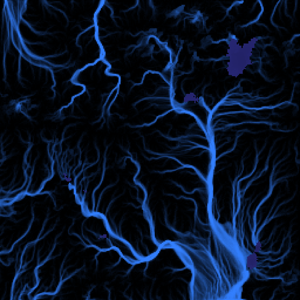
The stream map represents flowing water on the surface (streams and rivers). It stores the time-averaged particle positions on the map. Old information is discarded slowly.
The pool map represents non-flowing water on the surface (puddles, ponds, lakes, oceans). It stores the depth of the water on the map at a given position.
Note: The stream and pool maps are arrays with the same size as the height-map.
These maps are generated and coupled by particles, which move water around. Introducing these hydrology maps also gives us time-dependent information, allowing particle interaction while still simulating them individually. Particles can interact by using these maps to derive the parameters that influence their movement.
Note: The stream map is being displayed after passing through a shaping function (ease-in-out) and rendered on the terrain based on this. For more thin / crisp streams (or to ignore lower values in broad, flat areas), this can be modified or thresholded.
Water as a Particle
Water is represented by a discrete packet (“particle”), that has a volume and moves across the terrain surface. It has a number of parameters which influence exactly how it moves (friction, evaporation rate, sedimentation rate, etc).
This is the main data structure used to simulate hydrology. Particles are never stored but only used to interact between the height, stream and pool maps.
Note: The particle concept is explained in more detail in a previous blog post here (and countless other resources).
Hydrology Cycle and Map Coupling
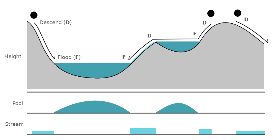
The maps are coupled to each other through the hydrology cycle. A hydrology cycle consists of the following steps:
- Spawn a particle on the terrain
- Descend the particle on the height-map and erode (i.e. Simple Particle-Based Hydraulic Erosion).
- If a particle stops or enters an existing pool, then attempt to create a pool on the map with its volume or add its volume to the pool by flooding.
- If a pool overflows, move a particle with the overflow volume to the drainage point and descend.
- The particle dies when it runs out of volume (by pooling or evaporation) or exits the map.
- Spawn a new particle and repeat.
There are only two algorithms for the entire system: Descend and Flood. Descending particles change the stream map, while flooding particles change the pool map. These algorithms are described in detail below.
Implementation
In the following, I will explain the full implementation of the system used to generate the results with code samples.
Note: I will only present the relevant portions of the code. More details can be found on the Github repo. All relevant portions of the code are in the file “water.h”.
Particle Class
The particle struct “Drop” is identical to that in the previous erosion system. Descend and flood are now members of the struct, as they act only on a single particle at a time.
struct Drop{

  //... constructors

  int index;                         //Flat Array Index
  glm::vec2 pos;                     //2D Position
  glm::vec2 speed = glm::vec2(0.0);
  double volume = 1.0;
  double sediment = 0.0;

  //... parameters
  const double volumeFactor = 100.0; //"Water Deposition Rate"

  //Hydrological Cycle Functions
  void descend(double* h, double* stream, double* pool, bool* track, glm::ivec2 dim, double scale);
  void flood(double* h, double* pool, glm::ivec2 dim);
};
An additional parameter is the volume factor, which determines how flooding translates volume into water level.
Descend Algorithm
The descend algorithm is almost the same as simple particle erosion. It takes an additional input “track”, an array where it writes all the positions that it visits. This is for constructing the stream map later.
void Drop::descend(double* h, double* stream, double* pool, bool* track, glm::ivec2 dim, double scale){

  glm::ivec2 ipos;

  while(volume > minVol){

    ipos = pos; //Initial Position
    int ind = ipos.x*dim.y+ipos.y; //Flat Array Index

    //Register Position
    track[ind] = true;

    //...
  }
};
The parameter set is modified by the stream and pool maps:
//...
  //Effective Parameter Set
  double effD = depositionRate;
  double effF = friction*(1.0-0.5*stream[ind]);
  double effR = evapRate*(1.0-0.2*stream[ind]);
//...
Note: I found this parameter modification to work well.
In the previous system particles would only break from this loop (and die) if evaporated completely or if they went out of bounds. Now two additional break conditions are included:
//... nind is the next position after moving the particle

  //Out-Of-Bounds
  if(!glm::all(glm::greaterThanEqual(pos, glm::vec2(0))) ||
     !glm::all(glm::lessThan((glm::ivec2)pos, dim))){
       volume = 0.0;
       break;
  }

  //Slow-Down
  if(stream[nind] > 0.5 && length(acc) < 0.01)
    break;

  //Enter Pool
  if(pool[nind] > 0.0)
    break;

//...
If the particle is not being accelerated sufficiently and it is surrounded by other particles, or it directly enters a pool, it will prematurely end its descent with all of its remaining volume and transition to the flood algorithm.
Note: The out-of-bound condition also sets the volume to zero, so particles don’t transition to the flood algorithm.
Flood Algorithm
A particle with remaining volume can perform a flood at its current position. This happens if it stops descending (no acceleration) or enters an existing pool.
The flood algorithm translates the particle’s volume into a raised water level by changing the pool map. The approach is to incrementally raise the water level by fractions of the particle’s volume using a “testing plane”. As the water level rises, the particle volume is lowered.
At every step we perform a flood-fill from the particle’s position (i.e. recursively test neighbors), adding all positions that are above the initial plane (current water level) and below the testing plane to a “flood-set”. This is the region of our terrain that is part of our pool.
During the flood-fill we test for drain points. These are points in our flood-set below the testing plane AND the initial plane. If we find multiple drains, we take the lowest.
void Drop::flood(double* height, double* pool, glm::ivec2 dim){

  index = (int)pos.x*dim.y + (int)pos.y;
  double plane = height[index] + pool[index];  //Testing Plane
  double initialplane = plane;                 //Water Level

  //Flood Set
  std::vector<int> set;
  int fail = 10; //Just in case...

  //Iterate while particle still has volume
  while(volume > minVol && fail){

    set.clear();
    bool tried[dim.x*dim.y] = {false};

    //Lowest Drain
    int drain;
    bool drainfound = false;

    //Recursive Flood-Fill Function
    std::function<void(int)> fill = [&](int i){

      //Out of Bounds
      if(i/dim.y >= dim.x || i/dim.y < 0) return;
      if(i%dim.y >= dim.y || i%dim.y < 0) return;

      //Position has been tried
      if(tried[i]) return;
      tried[i] = true;

      //Wall / Boundary of the Pool
      if(plane < height[i] + pool[i]) return;

      //Drainage Point
      if(initialplane > height[i] + pool[i]){

        //No Drain yet
        if(!drainfound)
          drain = i;

        //Lower Drain
        else if( pool[drain] + height[drain] < pool[i] + height[i] )
          drain = i;

        drainfound = true;
        return; //No need to flood from here
      }

      //Part of the Pool
      set.push_back(i);
      fill(i+dim.y);    //Fill Neighbors
      fill(i-dim.y);
      fill(i+1);
      fill(i-1);
      fill(i+dim.y+1);  //Diagonals (Improves Drainage)
      fill(i-dim.y-1);
      fill(i+dim.y-1);
      fill(i-dim.y+1);
    };

    //Perform Flood
    fill(index);

    //...
Note: This uses a recursive eight-way flood fill for simplicity. This can be implemented more efficiently in the future.
Once the flood-set and drains have been identified, we modify the water-level and the pool map.
If a drain is found, we move the particle (and its “overflow” volume) to the drain point so it can begin descending again. The water-level is then lowered to the height of the drain.
    //...

    //Drainage Point
    if(drainfound){

      //Set the Particle Position
      pos = glm::vec2(drain/dim.y, drain%dim.y);

      //Set the New Waterlevel (Slowly)
      double drainage = 0.001;
      plane = (1.0-drainage)*initialplane + drainage*(height[drain] + pool[drain]);

      //Compute the New Height
      for(auto& s: set) //Iterate over Set
        pool[s] = (plane > height[s])?(plane-height[s]):0.0;

      //Remove some sediment
      sediment *= 0.1;
      break;
    }

    //...
Note: When lowering the water-level due to drainage, I found that it works best to do so slowly with a drainage factor. Also, removing some sediment helps too.
This has the effect that new particles entering a full pool have their volume transported immediately to the drain point, as if adding the volume to the pool forced the same volume to leave the pool.
If no drain is found, we compute the volume under the testing plane and compare it to the particle’s volume. If it is smaller, we remove the volume from the particle and adjust the water level. The testing plane is then raised. If it is larger, the testing plane is lowered. This is repeated until the particle has no volume left or a drain point is found.
    //...

    //Get Volume under Plane
    double tVol = 0.0;
    for(auto& s: set)
      tVol += volumeFactor*(plane - (height[s]+pool[s]));

    //We can partially fill this volume
    if(tVol <= volume && initialplane < plane){

      //Raise water level to plane height
      for(auto& s: set)
        pool[s] = plane - height[s];

      //Adjust Drop Volume
      volume -= tVol;
      tVol = 0.0;
    }

    //Plane was too high and we couldn't fill it
    else fail--;

    //Adjust Planes
    float approach = 0.5;
    initialplane = (plane > initialplane)?plane:initialplane;
    plane += approach*(volume-tVol)/(double)set.size()/volumeFactor;
  }

  //Couldn't place the volume (for some reason)- so ignore this drop.
  if(fail == 0)
    volume = 0.0;

} //End of Flood Algorithm
The plane height is adjusted proportionally to the volume difference, scaled by the pool surface area (i.e. set size). By using an approach factor, you can increase stability of how the plane reaches the correct water level.
Erosion Wrapper
A world class contains all three maps as flat arrays:
class World {
public:
void generate(); //Initialize
void erode(int cycles); //Erode with N Particles
//...
double heightmap[256*256] = {0.0};
double waterstream[256*256] = {0.0};
double waterpool[256*256] = {0.0};
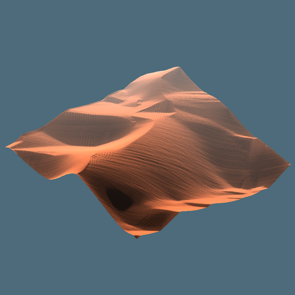
};Note: The height-map is initialized using Perlin-Noise.
An individual hydrology step for a single particle consists of:
//...

//Spawn Particle
glm::vec2 newpos = glm::vec2(rand()%(int)dim.x, rand()%(int)dim.y);
Drop drop(newpos);

int spill = 5;
while(drop.volume > drop.minVol && spill != 0){

  drop.descend(heightmap, waterstream, waterpool, track, dim, scale);

  if(drop.volume > drop.minVol)
    drop.flood(heightmap, waterpool, dim);

  spill--;
}

//...
The “spill” parameter determines how many times a particle can enter a pool and leave a pool again before it is simply killed. Particles otherwise die when their volume is depleted.
Note: Particles rarely enter and exit more than one or two pools before they evaporate entirely on the descend steps, but I added this just in case.
The erode function wraps this and performs the hydrology steps for N particles and updates the stream map directly:
void World::erode(int N){

  //Track the Movement of all Particles
  bool track[dim.x*dim.y] = {false};

  //Simulate N Particles
  for(int i = 0; i < N; i++){

    //... simulate individual particle

  }

  //Update Path
  double lrate = 0.01;  //Adaptation Rate
  for(int i = 0; i < dim.x*dim.y; i++)
    waterstream[i] = (1.0-lrate)*waterstream[i] + lrate*((track[i])?1.0:0.0);

}
The track array is passed to the descend function here. I found that tracking the movement of multiple particles simultaneously, and updating in this fashion gives better results in the stream map. The adaptation rate determines how quickly old information is discarded.
TREES
Just for fun, I added trees to see if I could enhance the erosion simulation some more. These are stored in the world class as a vector.
Trees spawn randomly on the map in the absence of pools or strong streams, and where the terrain isn’t too steep. They also have a chance to spawn other trees near themselves.
As they spawn, they write to a “plant density” map in a certain radius around them. A high plant density lowers the mass-transfer between descending particles and the terrain. This is to simulate roots holding the ground together.
//... descend function
double effD = depositionRate*max(0.0, 1.0-treedensity[ind]);
//...
Trees die if they are in a pool or if the stream beneath them is too powerful. They also have a random chance to die.
Note: You can find the tree model in the file “vegetation.h” and the function “World::grow()”.
Other Details
The results are visualized using a homemade OpenGL wrapper, that you can find [here].
Results
Particles can be spawned on the map according to whatever distribution you like. For these demonstrations, I spawned them uniformly on maps of size 256×256.
The resulting simulation is highly dependent on the choice of initial terrain, as you will see below. The system is capable of imitating a wide variety of natural phenomena. One which I haven’t been able to adequately capture is canyons. This would possibly require very long-time, slow simulation.
Other phenomena such as waterfalls, meandering, deltas, lakes, swelling and more can be observed.
The system also does very well to distribute streams and pools in places where lots of rain accumulates instead of arbitrary placement. The generated hydrology is therefore tightly coupled to the terrain.
Stream Sharpening Effect Comparison
To compare the difference that coupling the map into the erosion system makes, we can simulate the hydrology on the same map while activating different effects.
I simulated the same terrain three times:
- Particle based erosion (base erosion), extracting stream and pool maps. Pools still affect the generation
- Base erosion with parameters modified by the hydrological maps (coupled erosion)
- Coupled erosion with parameters modified by the hydrological maps and trees affecting erosion
Note: This a relatively chaotic system, and what kind of hydrology appears depends highly on the terrain. It is difficult to find a “very representative” sample terrain.
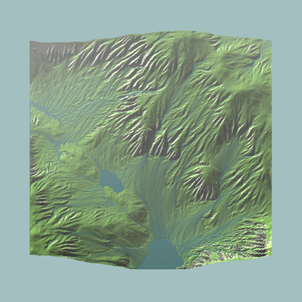
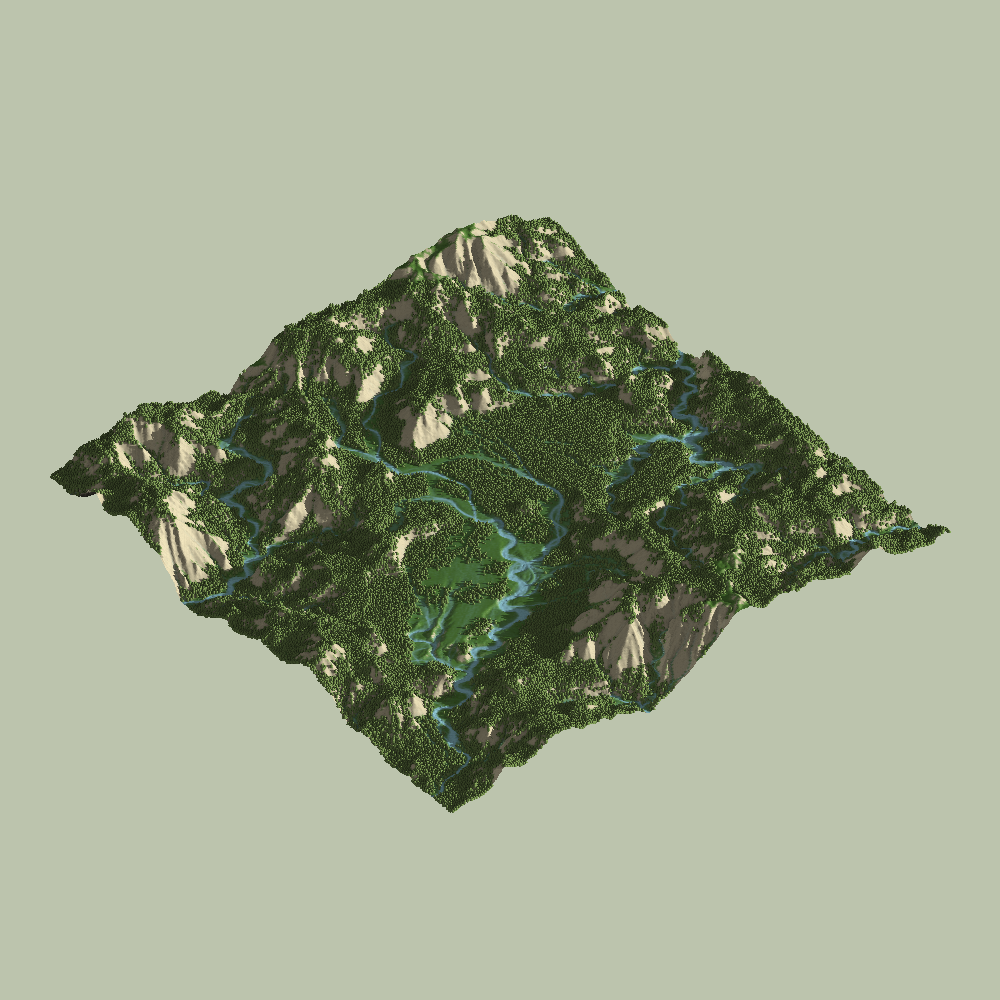
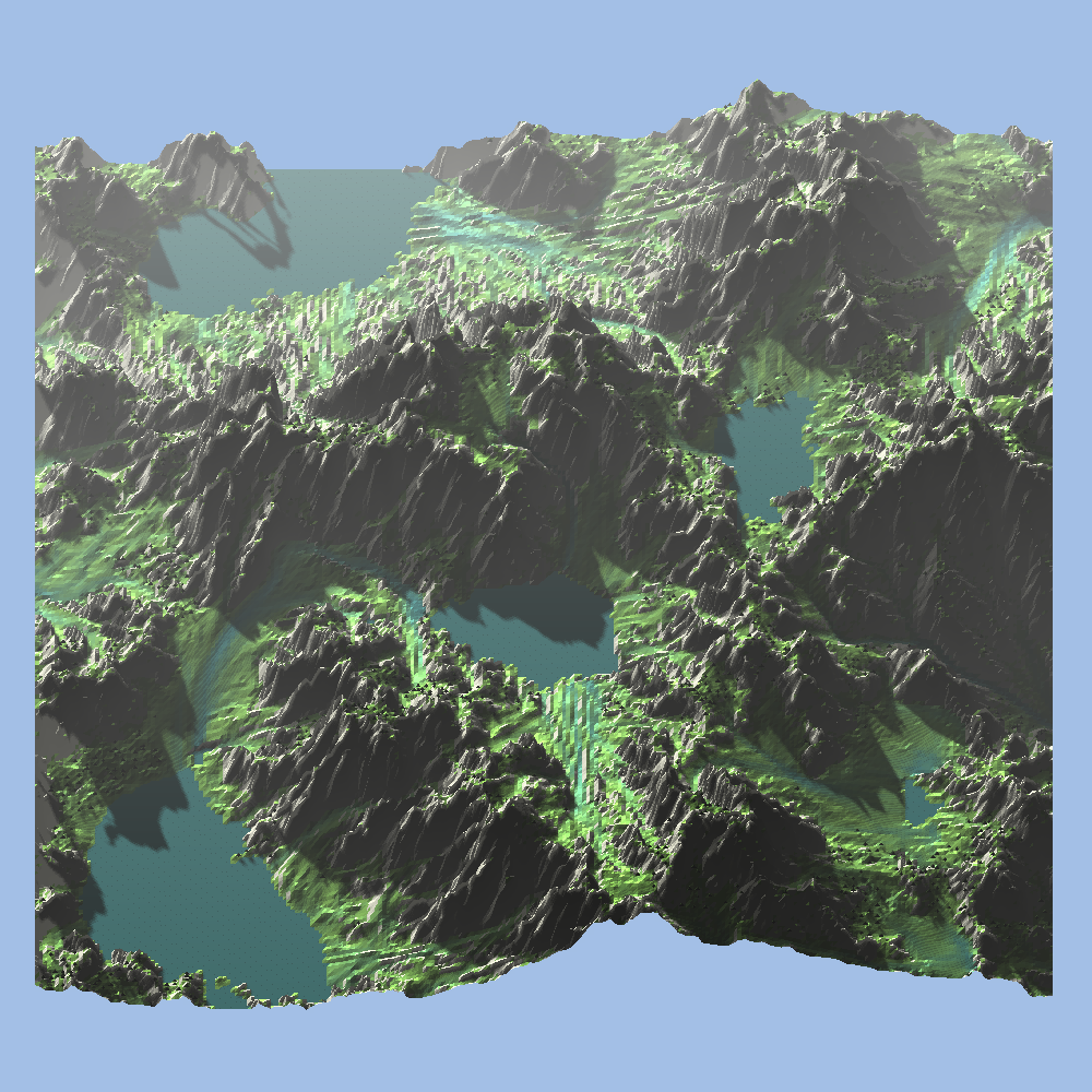
Terrain Render of the Base System 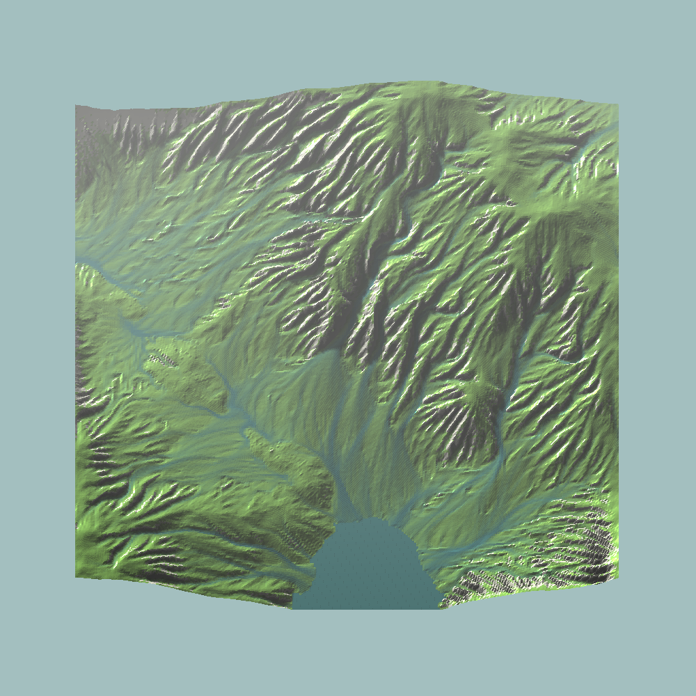
Terrain Render of the Coupled System 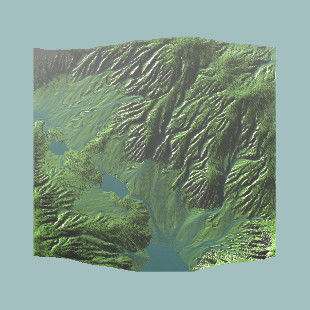
Terrain Render of the System with Trees
One interesting observation is that coupling the hydrology maps back into the particle parameters indeed sharpens the river paths. Particularly in the flat regions, the particles are less spread out and converge more in a few, stronger paths.
Lower friction and evaporation rate successfully makes the particles prefer established paths.
Other effects are more noticeable when looking at the terrain directly.
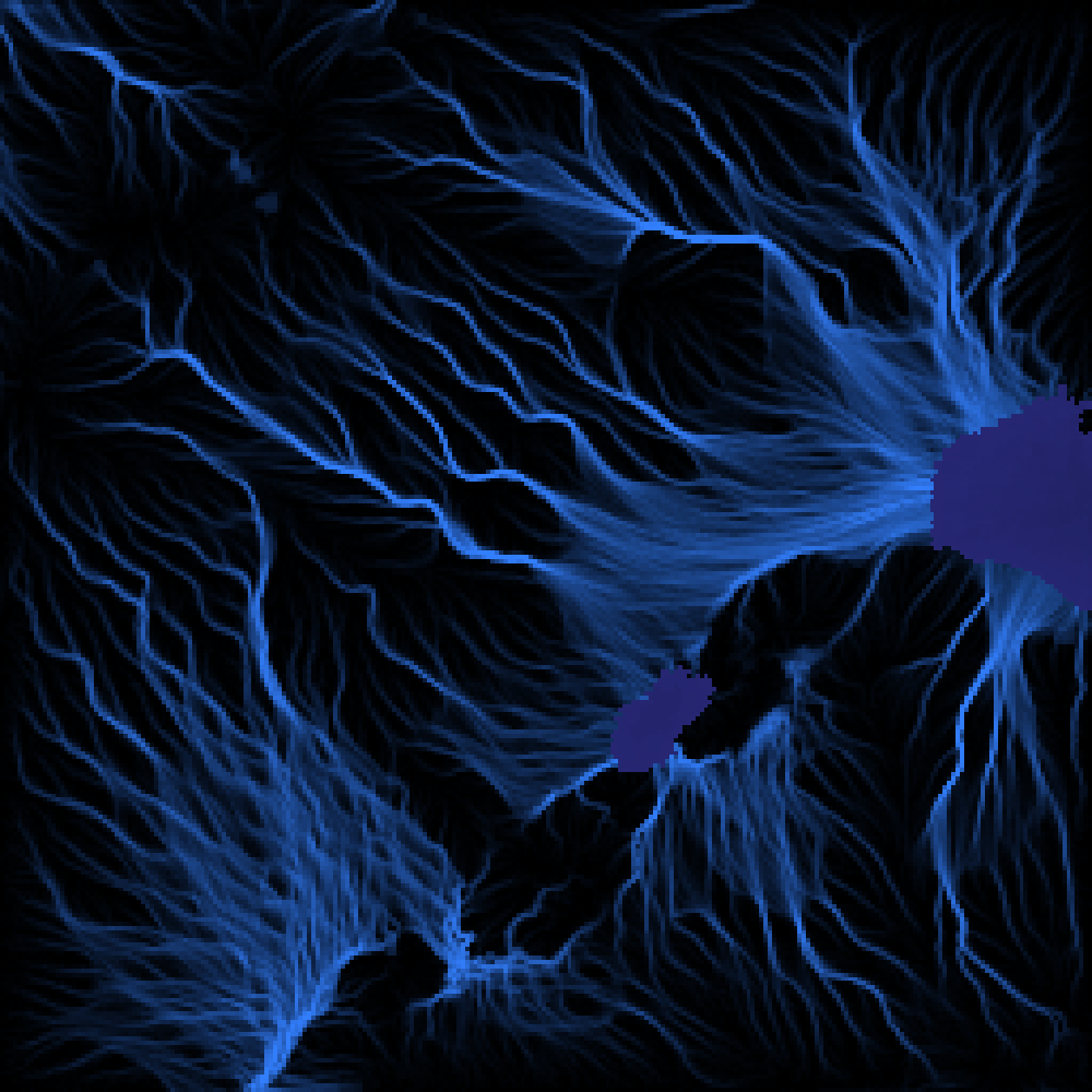
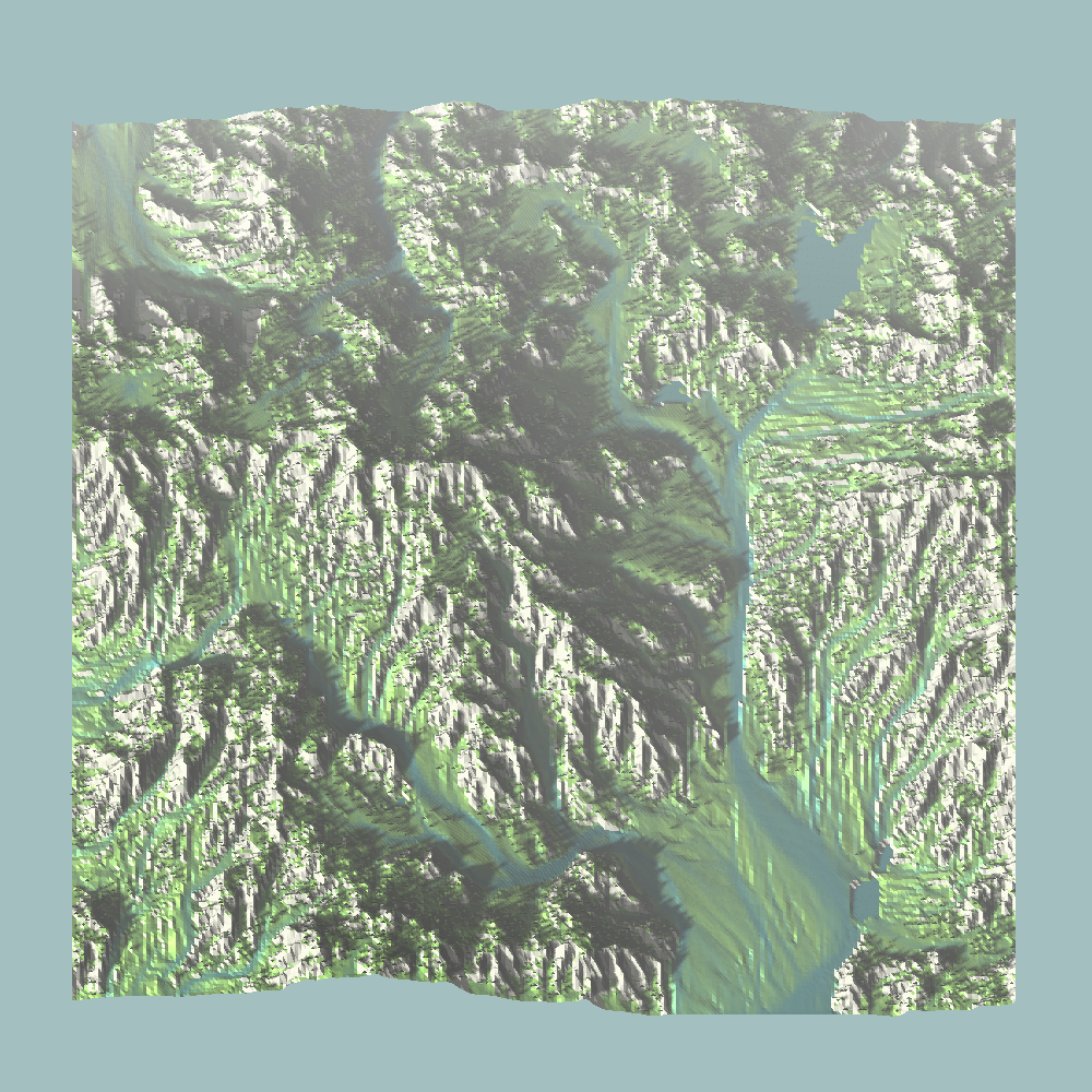
Hydrology Map of the Base System 
Hydrology Map of the Coupled System 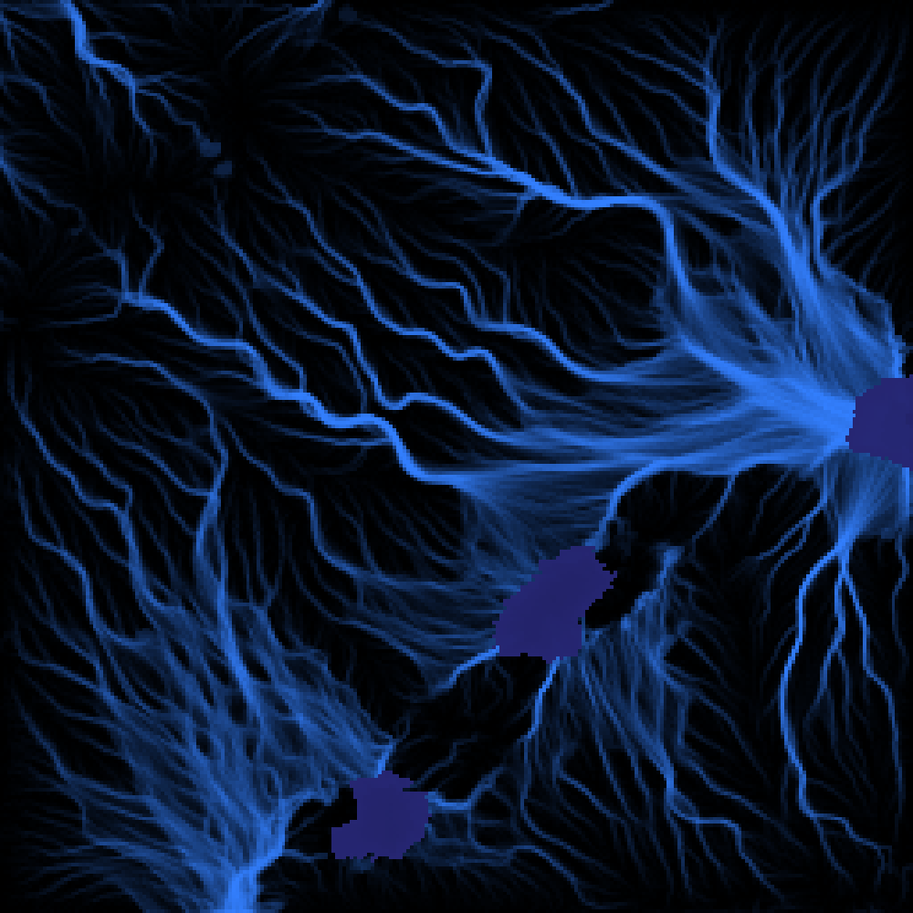
Hydrology Map of the System with Trees
Note: These results were generated with exactly 60 seconds of simulation time.
Trees had a small additional effect on sharpening. They enhanced the streams carving distinct paths in the steeper regions. They force the streams to remain in already established paths and thus reduce meandering. How you place trees can thus affect the water movement.
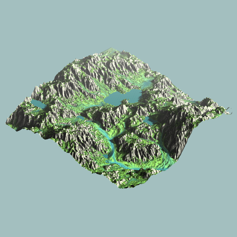
Pooling Effects
The pooling system works well and allows multiple bodies of water to exist on the same terrain at different heights. They can also effectively drain into each other and be emptied.
Note: I have seen a few seeds were 3 lakes successively drain into each other, but I didn’t want to spend a long time running simulations to find one for this article. I have already generated too many pictures and videos (lmao).
Occasionally, the height level of the pool will jump around. I think this happens when the water level is near the drainage level and lots of water is being added. This is reduced by lowering the drainage rate in the flood function.
After another minute of generation, some more pools established themselves. 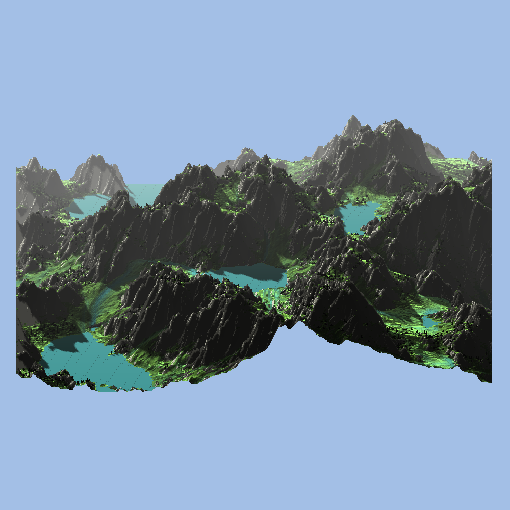
At a steeper angle, the height difference in the pools is more visible. 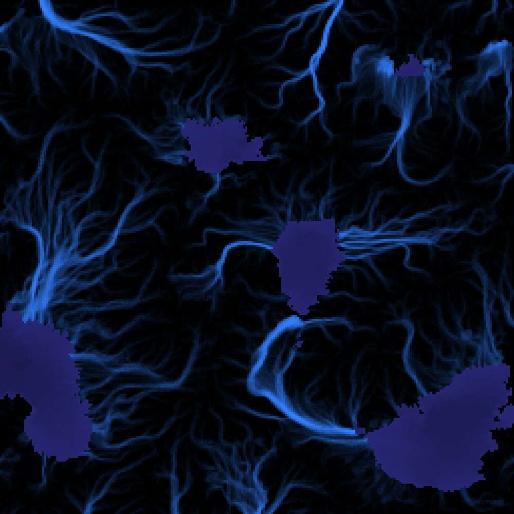
The hydrology map clearly shows the middle pool draining into the lower pool.
The flooding algorithm leads to pools seeing a “wall” at the boundary of the map. This can be seen in the images above.
One potential improvement would be to add a sea level parameter to the world, so that pools observe a drain at the map boundary at sea level and otherwise simply flow over.
Simulation Speed
The time for an individual descend and flood step varies from particle to particle, but remains on roughly the same order of magnitude (~ 1 microsecond). With established streams, particles move faster across the map.
Flooding time scales with the size of the pool as the flood fill operation is the most expensive step. Larger pools means more area for which to increase the water level. Large pools definitely represent the system bottleneck. If you have ideas for improving the speed, please let me know.
Descending time scales with the size of the map and a number of other parameters, including friction and evaporation rate.
All videos in this article were recorded in real time, so the simulation is fast overall.
Note: Shortly after publishing this article, I made a small change in how the surface normals are computed that increased simulation speed. The effect is definitely noticeable when running the simulation, but hard to benchmark due to large variations in the run times of descend and flood. I estimate that simulation speed is doubled.
More Nice Videos
The following videos were made after speed improvement.
I could do this forever.
Summary and Future Work
This simple technique is still based on particles, but successfully captures a number of additional effects. It offers a shortcut method for simulating large-scale water movement without full fluid dynamics simulation. It also works well with an intuitive data representation of water.
In the simulations, we can observe river meandering, waterfalls, lakes and lake draining, rivers splitting into wide deltas in flat regions, etc. We thus get very nice dynamic effects, with information about water depth and flow.
It would be interesting to include different types of soil in the form of a soil map, from which one can source erosion parameters.
It would also be easy to modify the tree system to have different types of plants that hold the ground together.
It’s hard to capture the diversity of the generated results in a few videos and pictures, so you should really try this yourself: it’s very fun. I recommend playing around with initial map parameters, including the octaves of noise and the map scale.
If you have any questions or comments about this, feel free to contact me. I worked quite intensely on this, so my brain is very fried and I’m sure I missed some interesting aspects.
Other Modeling Thoughts
This model is easily adaptable to non-uniform grids (e.g. arbitrary triangle, hexagonal, etc.) by adapting the method for computing the surface normal (for particle movement) and the flood-fill operation (simply adjust the neighborhood).
One key issue is the choice of when a particle transitions from its particle state to the pool state. This transition could be considered a transition from a non-viscous to a viscous flow and could be set based on Reynolds-Number. Currently this is somewhat arbitrary.
Another issue is the lack of flow within pools. Particles are transported immediately to the outlet, but in reality there would be a time-delay based on the shape of the pool. This could be modeled based on residence time of the pool or based on the wave propagation speed in the pool (e.g. shallow-water equations) multiplied the distance from the entry point to the drain.
I believe that changing the surface representation and how the surface normals are computed has a significant on particle motion. Currently, normals are computed within a very small neighborhood, leading to strong ridges forming. If the neighborhood with high normals are computed is extended, I expect fewer ridge artifacts to appear. This could be done e.g. with a least squares regression to locally approximate the surface as a plane, or by computing a poisson surface over the entire grid (might be expensive).