Note: The full source-code used to generate all visualizations is available on Github here, unless specified otherwise. More modern iterations of the code will be discussed at the end.
Preface
Since the publication of my article on Procedural Hydrology through particle-based erosion simulation and the release of the source-code as SimpleHydrology over 3 years ago, the reach of the concept has far exceeded my expectations, becoming one of the most popular open-source projects under the topic hydrology on Github, with around 2^9 (= 512) stars at the time of this publication.
I am particularly grateful for the countless conversations I have had over E-Mail and Reddit, particularly with the r/proceduralgeneration community, discussing the beauty, complexity and merit of these simulations, and it has inspired me to dive deeper into topics of simulated and procedural geomorphology.
SimpleHydrology as an implementation has since been a baseline for my geomorphology simulations, both visually but also in terms of my procedural generation ideal:
Maximize emergent behavior and minimize complexity through well defined and comprehensible rules
In the time since the original publication, SimpleHydrology has gone through many iterations, improved by addressing its core deficiencies, but also finding the most effective way to boost the emergent output space with only minimal new rules and complexity. That is what this article is about.
This has been a long time coming. For anybody who has been following this blog over the years, thank you for reading, and I hope you can appreciate the work that goes into these projects. It is quite difficult to “make time” next to full-time jobs and other real life considerations, even when I find that musing about these designs occupies most of my daily mental bandwidth. I hope you enjoy reading this as much as I enjoy designing and writing about it!
Introduction
This article is a follow-up article to Procedural Hydrology. In it, I will lay out my criticisms of the implementation, and how they are addressed to improve the overall quality of the simulation.
Additionally, I will explain the main conceptual improvement that has been made to the SimpleHydrology system: Meandering Rivers.
Through the introduction of a low complexity change (the computation and conservation of momentum), a large amount of emergent complexity can be effected, resulting in beautiful and realistic time-lapse behavior of meandering rivers, dry stream-beds and soil being pushed around.
If you would like to know how to get effects similar to these in your erosion simulations, this article will lay it all out!
In the two videos above, you can see a time-lapse (5x speed-up) of the meandering river simulation. How this works will be discussed in more detail below.
Procedural Hydrology: Retrospective
It is not necessary to read the original Procedural Hydrology article to learn about Meandering Rivers in particle-based erosion simulations, but this section is a retrospective, which addresses insights and improvements to the code that apply generally to erosion simulation code. The original article has more detailed explanations and implementation examples, which will be referenced here. Skip at your own peril.
Procedural Hydrology in a Nutshell…
Procedural Hydrology is a particle-based hydraulic erosion simulation with streams and pools in a 2.5D-Domain (i.e.: on a height-map). These streams and pools, represented by stream and pool maps respectively, were designed to couple the particles’ behavior more tightly to the terrain and yield more realistic morphology. It works as follows:
Water particles are spawned, distributed randomly over the terrain, and descending by the law of gravity (think: rain). Particles have mass and thereby individual momentum, so that they can escape small, local terrain minima. The paths of particles are tracked in the stream-map and exponentially averaged, approximating a dynamic probability distribution for particle positions on the grid.
An equilibrium mass function takes the current state of the particle (speed, local terrain slope, etc.) and determines the amount of mass the particle can suspend at equilibrium. The equilibrium value is approached iteratively by the actual value, by transferring sediment between the particle and the terrain using a linear mass-transfer rate.
Finally, before a particle dies, it can attempt to “flood”, by which it will take any remaining, non-evaporated volume, and add it to the pool map to signify stagnant water on the terrain. It does so using a flood-fill operation over the terrain.
The simulation is defined by two processes:
The Particle Motion-Law and Mass-Transfer-Law.
Making these two processes dependent not only on the height-map, but also the pool-map and the stream-map (i.e.: other particles) is what lets SimpleHydrology be more realistic than simple hydraulic erosion. Still, there are certain aspects which I would do differently today…
Note: I have written about this before, but I still believe that almost any surface-dynamic geomorphological phenomenon can be simulated through the combination of a motion-law and mass-transfer-law in a particle-based system; even those which would be typically solved through cellular automata in a Eulerian Frame. This is possible as long as particle-motion can be designed to move along the characteristics of the relevant dynamic law for energy and mass transfer. It has worked out for me so far.
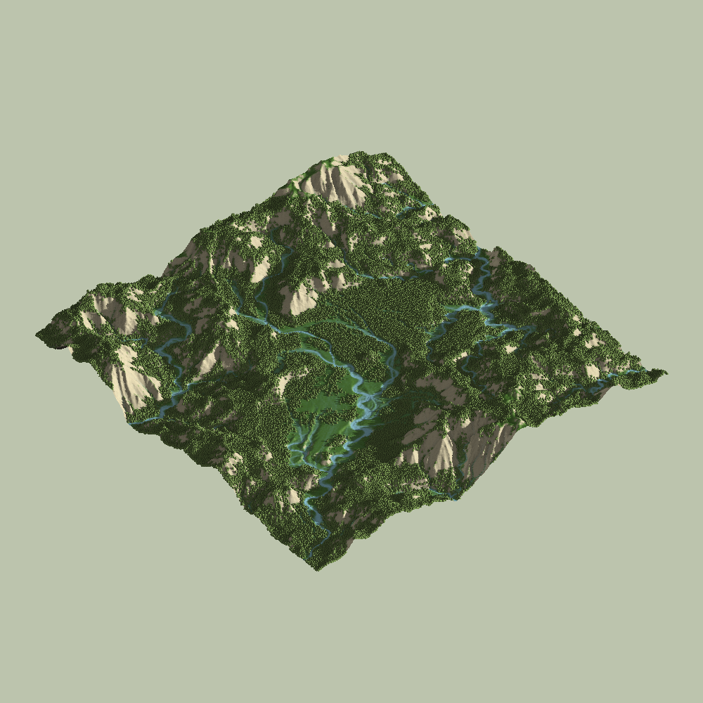
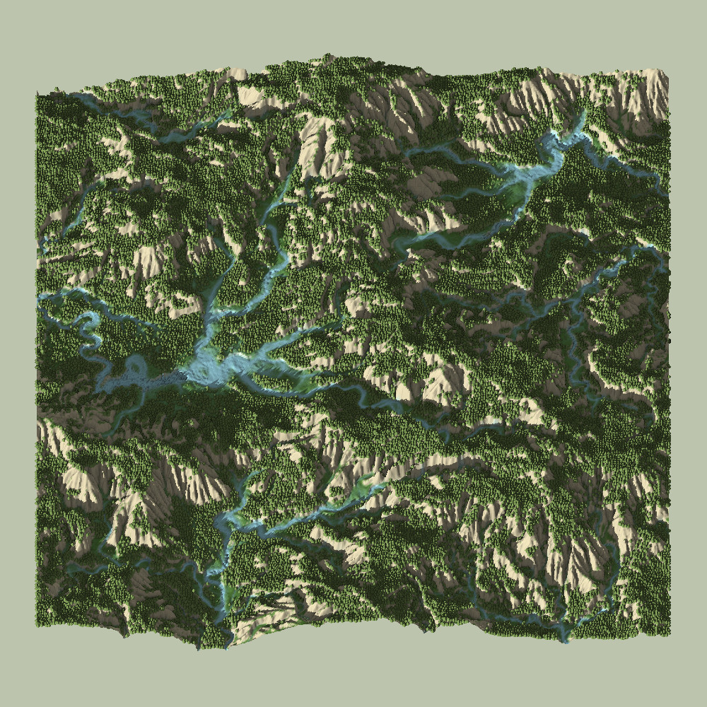
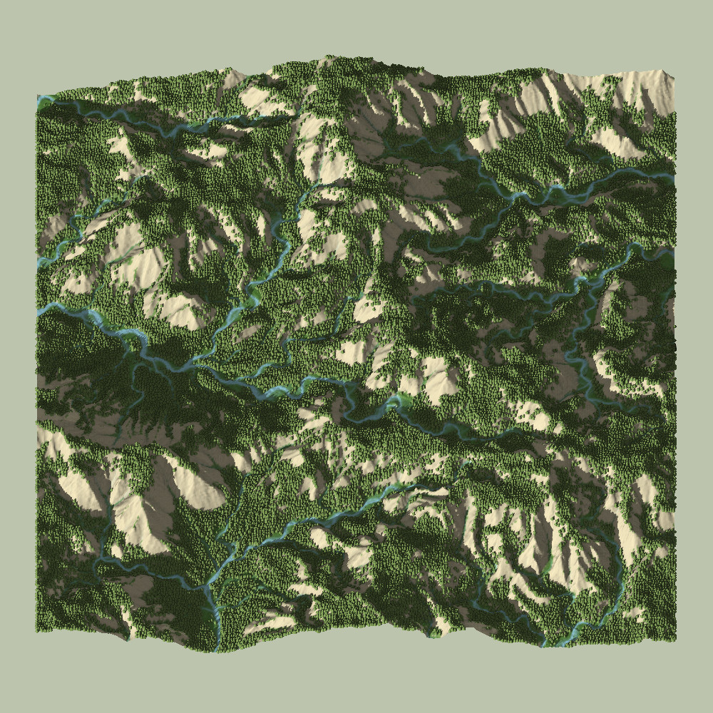
Observe the images above. On the left is the old system, while the right contains all of the improvements I have made over the years. Graphical improvements aside (specularity, distance-fog, SSAO, non-billboard trees), the image on the left has a number of artifacts which the image on the right doesn’t have.
The artifacts, their causes and their fixes are explained below, in no particular order.
Criticism 1: Natural Smoothing
Probably the first observation is that the terrain on the left looks very jagged, with deep ridges. Hydraulic erosion has the self-reinforcing property that deep ridges tend to get deeper, as gravity moves more particles down the steeper slope, leading to more erosion, and so on.
This is not an invalid morphology, as deep-ridged mountains are common in places like Hawaii or Southern China. My issue was that I had no control over it.
At the time, I considered introducing a smoothing function (local averaging, gaussian blur, etc.) but thought that these were physically unrealistic and decided not to add them.
It was only 6 months after publication of SimpleHydrology that I began working on the SimpleWindErosion system, which necessitated the introduction of sand-pile dynamics and Angle of Repose for loose sediment.
It was only afterwards that I realized that rocky terrain naturally has the same mechanism, with particles (rocks) falling into the ridges from above through thermal erosion, acting as an effective and natural local smoothing filter.
Thermal Erosion and Sediment Avalanching is essential for realistic Hydraulic Erosion Simulations.
This natural sediment settling process is a well-described phenomenon which gives mountains and hills characteristic slopes and helps enforce the fractal-like appearance.
In the simulation, this has the effect that ridges can never become arbitrarily deep, since this increases the slope and forces material to naturally fall from above. Finally, different materials can be given different angles of repose, adding an additional layer of depth and control.
The rate of thermal erosion can also be reduced when simulating erosion in climates without freeze-thaw cycles.
Note: An up-to-date implementation of avalanching is here.
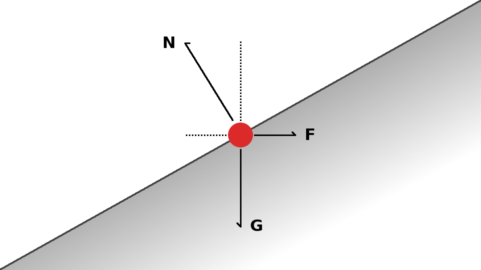
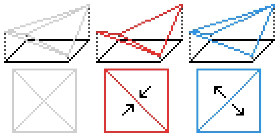
Criticism 2: Surface-Normal
Meshing a rectangular-grid height-map with triangles has one seemingly trivial but incredibly relevant issue: The choice of orientation for the triangles is arbitrary and affects the “graphical slope” of the surface.
This is because the convex hull of the four corner-points of a cell is almost never a quad, but a tetrahedron with 4 triangle faces: two above and two below. That’s a complicated way of saying that you have to choose which pair of triangles you want to represent your surface, affecting local slope.
At the time, I decided that the simulation and its visualization should not be separate, if possible. So far so good.
I then for some reason decided that the terrain surface should be equal to the surface-mesh, i.e. the simulation slope would be equal to the mesh slope (graphical slope).
This was a mistake, conceptually and computationally.
The arbitrary nature of the orientation introduced directional artifacts which were difficult to diagnose and remove. In trying to fix them, I computed the normal from both orientations simultaneously. Relying on the triangle slope required multiple cross-product and many normalization operations, which were expensive and slowed down the simulation, especially after removing the artifacts, doing twice the work.
Finally, inside any of the four regions of the projected tetrahedron (see image above, bottom left), the slope would be constant and there was no local variation, with sharp changes in slope at the boundaries between these internal triangles. All around terrible.
The fix was realizing that the normal-vector of a continuous surface can be computed from the surface-gradient. An arbitrary precision, continuous approximation of the surface-gradient with any choice of support points can be computed using finite differences. This was not only computationally much more efficient, but allowed for granular control of the accuracy vs cost trade-off at sub-pixel values, achieving higher levels of detail.
The thinking that the graphics and simulation should not be separated was not bad in principle – I had just chosen the wrong end to be in charge. Instead of using the surface-normal properties of the mesh for simulation, I instead now use a normal-map, computed using the simulation’s finite-difference method, for lighting the terrain.
Here is a working C++20 example implementation:
// Surface Map Constraints

template<typename T>
concept surface_t = requires(T t){
  { t.height(glm::ivec2()) } -> std::same_as<float>;
  { t.oob(glm::ivec2()) } -> std::same_as<bool>;
};

// Finite-Differences Gradient Method

template<surface_t T>
const static inline glm::vec2 gradient(T& map, glm::ivec2 p){

  glm::vec2 pxa = p;
  if(!map.oob(p - glm::ivec2(1, 0)))
    pxa -= glm::ivec2(1, 0);

  glm::vec2 pxb = p;
  if(!map.oob(p + glm::ivec2(1, 0)))
    pxb += glm::ivec2(1, 0);

  glm::vec2 pya = p;
  if(!map.oob(p - glm::ivec2(0, 1)))
    pya -= glm::ivec2(0, 1);

  glm::vec2 pyb = p;
  if(!map.oob(p + glm::ivec2(0, 1)))
    pyb += glm::ivec2(0, 1);

  // Compute Gradient

  glm::vec2 g = glm::vec2(0, 0);
  g.x = (map.height(pxb) - map.height(pxa))/length(pxb-pxa);
  g.y = (map.height(pyb) - map.height(pya))/length(pyb-pya);
  return g;

}

// Surface Normal from Surface Gradient

template<surface_t T>
const static inline glm::vec3 normal(T& map, glm::ivec2 p){

  const glm::vec2 g = gradient(map, p);
  glm::vec3 n = glm::vec3(-g.x, 1.0f, -g.y);
  if(length(n) > 0)
    n = normalize(n);
  return n;

}
Note: This code snippet utilizes C++20 concepts so that it can generically operate on any type which implements the height() and oob() methods, with only one square root and no cross products. This code is taken from here.
Criticism 3: Constant Time-Step
The next most apparent issue with the height-map is that the terrain appears quite noisy, and as the simulation runs, holes and spikes are created and filled again. The reason for this is quite simple: the constant time-step.
As particles move, gaining or losing speed based on the laws of motion, they traverse the grid’s cells. The issue is that:
With a constant time-step, there is no guarantee that a particle will land in a neighboring cell after each step.
This had two effects: Particles were capable of “tunneling through” and “leaping over” terrain features, and the effective slope computation and thus mass-transfer law was no longer local. These effects could average out over time, but the simulation would look noisy and unrealistic as it progressed. Example:
This is fixed by normalizing the effective speed of each particle has to be equal to the cell-width, so that there is a guarantee that a particle will land in a neighboring cell. Thereby, mass can no longer tunnel through or leap over terrain. To then adjust the motion-law and mass-transfer-law rates, the time-step parameter (dt) has to be scaled by the ratio of the particle speed to the cell-width.
Note: This effectively reinterprets the particle speed more as a time-dilation parameter than an actual velocity over the map, but makes the simulation stable and smooth.
Criticism 4: Flood-Fill Pooling
The stream-map was a great idea. The pool-map was not so great, but what made it really terrible was that I decided to use flood-filling for updates. Allow me to explain.
Incrementally distributing the remaining volume of a water droplet, equally over the surface of a body of water, determined by a complex flood-fill, turned out to be computationally expensive. Now do this for hundreds of droplets per time-step, as lakes grow larger and larger, and you can see the complexity scaling problem.
Flood-filling was also not a good idea conceptually, since the surface height equilibrium of any real body of water does not propagate instantly, but with a finite wave-speed. Flood-filling essentially decoupled the lake’s surface from the time-scale of the simulation.
The final issue was not getting lakes to fill, but to get them to drain. Determining drainage points on a constantly mutating, 2.5D basin boundary during the flood-fill was tremendously complex, with many edge cases (ba-dum-tss).
Drainage with flood-fills is what finally tipped the balance between implementation simplicity and emergent complexity towards the unreasonable, and the system was so fragile as to not be reasonably extensible.
At the end of my Procedural Hydrology article, I muse about what a good method would be to determine when the transition between flowing (particle) and stagnant (pool-map) water should take place. The answer? There is none. The question is far too ill-posed.
Dynamic Lakes are Difficult
I am sorry to say that I still don’t have the answer to this problem, but my previous one is definitely out of line with my procedural ideal.
I decided to remove lakes from the simulation entirely until I revisit them in the future, as I will (at some point) be tackling oceans, which behave in a more similar manner, and I might have more insights at that point.
I do have some ideas for how lakes could be done.
The concept takes inspiration from SoilMachine, my Multi-Layer Erosion Simulator. The pool map is effectively a static layer, permanently above the soil. Why don’t I treat it that way? It has a repose angle of zero, and can avalanche just like sediment. Water droplets contain soil and water. So I can define an equilibrium-based mass-transfer-law for the water volume, just like I do for the sediment, right? And of course, the particle would move different if it is on the surface of water.
That means that we no longer have to wrestle with incredibly ill-posed questions such as “when does water transition from a stream to a pool”. Instead, water is represented as in equilibrium between the particles and the map, coupling the particle motion to the terrain through a mass transfer / equilibriation law. When a particle flows over and out of a lake, it can carry that water with it naturally.
The only remaining challenge is defining the motion-law and the mass-transfer-law sensibly. Easier said than done. In the video above, I tried to do just that. That was about two months of work, but is still incomplete. It is much faster, more controllable, and has no edge cases. I am hopeful.
Criticism 5: Directionless Streams
The final criticism of Procedural Hydrology is that in shallow or low-slope regions of the map, the streams tend to “flatten out”, allowing them to braid nicely, but losing coherence and no longer acting like streams with a well-defined direction.
Just like with sediment avalanching, this can be a valid morphology in certain situations, like river deltas where the discharge rate becomes very low due to low flow rate spread over large areas. Still, the simulation lacked control over the coherence of streams in high discharge scenarios.
The issue arises from the fact that each particle’s motion does not affect the motion of any other particle: They are decoupled from each other.
This will be addressed in more detail in the following section on Meandering Rivers.
Additional Improvements
Here are additional improvements which don’t fall under the category of explicit criticisms, but rather optimizations and design choices.
1. Map-Cell Structure
Previously, I stored various properties of the map in separated arrays of basic C++ types. Instead of this, I now allocate a single array of a struct containing all properties.
float* height          = new float[WIDTH*HEIGHT]; // Heightmap Value
float* discharge       = new float[WIDTH*HEIGHT]; // Effective Discharge
float* discharge_track = new float[WIDTH*HEIGHT]; // Discharge Tracking Valu
float* rootdensity     = new float[WIDTH*HEIGHT]; // Vegetation Root Density
struct cell {
float height; // Heightmap Value
float discharge; // Effective Discharge
float discharge_track; // Discharge Tracking Value
float rootdensity; // Vegetation Root Density
};
cell* my_map = new cell[WIDTH*HEIGHT];Array of Struct > Struct of Array
(in this situation)
This is more cache-friendly since the data of a struct is stored contiguously, and it is more likely than not that you will be accessing different data-members at the same cell position than the same member of different cells.
This also easier to maintain; simply adding an additional member to your struct definition adds data to the map. In general, it allows for better decoupling of the map code from the erosion code and the introduction of convenience structures like iterators.
2. Discharge Function
The stream-map was originally intended to yield a dynamic value, characteristic of the volumetric flow through a particular point on the map. The volume of a particle would vary over its lifetime, and more particles would converge in high discharge areas of the map, which would affect the local motion- and mass-transfer-laws.
In order to generate the stream-map, I previously executed a boolean AND of the particle position and a particle-track map. After every particle has finished its motion, I would exponentially average the track-map with the stream-map.
Note: The previous implementation is here.
The issue with this implementation was that it had no realistic physical interpretation, despite my stated goal. In fact, I could not get it to work using the particle volumes, which is why I opted for the other implementation: it worked. This has been fixed since.
cell->discharge_track += drop.volume; // During Single Particle Descentfor(auto [cell, pos]: map){ // After All Particle Descent
cell.discharge = (1.0f-lrate)*cell.discharge + lrate*cell.discharge_track;
}const inline float discharge(glm::ivec2 p){ // Sampling Function
if(!map.oob(p))
return erf(0.4f*map.get(p)->discharge);
return 0.0f;
}In the new version, a discharge track value is accumulated over all particles at every time-step, giving the total volume which flowed through each cell. This value is subsequently exponentially averaged and passed through an error function to normalize the value to the range [0, 1).
Note that this introduces an additional parameter (the error-function characteristic scale) by which the activation of the discharge can be controlled.
Meandering River Simulation
It turns out that the change required to make particle-based hydraulic-erosion streams meander is quite minimal and non-invasive. This is well aligned with the principle of low complexity rules with high levels of emergence. In the following section, I will provide some context and finally present an implementation with code examples.
The Physics of Meandering
The Wikipedia-Article on Meandering states that a meander is caused by a higher flow-velocity on the outer bank of a river flowing around a curve, leading to more sediment being suspended by the flow at equilibrium. On the inner bank, the lower velocity leads to deposition of the excess sediment. Small disturbances in the linearity of the flow are thus self-enhancing, and will grow until a cut-off event occurs.
Minute-Earth on YouTube has a very concise explanation of the physics of meandering in video-form, describing the same phenomenon:
Interestingly, the Wikipedia article focuses primarily on how and why the flow has a velocity gradient when discussing the underlying physics, citing a balance between pressure (inwards) and centrifugal forces (outwards) leading to helical flow and sediment being moved across the bed of the river.
Note: You may notice that the simulation doesn’t define a velocity, in particular because we use a dynamic time-step to scale particle speed to the cell-width. Instead, we approximate the velocity as proportional to the discharge per unit-area, per unit-time.
So how do we introduce meandering into a particle-based hydraulic erosion simulation? There are two requirements:
1. Suspension Rate scales with Flow Velocity
The first requirement for meandering can already be satisfied by the simulation: A higher flow velocity leads to more suspension. This is realized using the discharge as a scaling factor for our equilibrium-mass function:
// Equilibrium Mass Function c_eq

float discharge = world.discharge(drop.pos); // Local Discharge Function
float entrainment = param.entrainment;       // Rate Parameter
float hdiff = world.height(drop.old_pos)-world.height(drop.pos);

float c_eq = (1.0f+param.entrainment*discharge)*hdiff;
if(c_eq < 0)
  c_eq = 0;
2. Flow Velocity increases at Outer Banks
The second requirement for meandering is to have a higher velocity on the outer banks of curved streams. This is where we come full-circle to the criticisms of the old Procedural Hydrology system: Each particle’s motion is decoupled from the motion of every other particle.
This effectively means that every particle has its own local momentum, but the stream as a whole does not, resulting in a lack of centrifugal forces. To meander, we will therefore:
Conserve Stream Momentum for Centrifugal Forces
Momentum Conservation
Note: To all CFD engineers reading this, prepare for hand-waving. I know that this is not true momentum conservation, but a very basic approximation which is suited to the procedural nature of the simulation and provides excellent results. An analysis of why this works and what it is actually modeling would be interesting.
In order to conserve momentum and couple the motion of all particles, we use an additional momentum-map.
The momentum-map is given by the exponential average (over time-steps) of the cumulative momentum of all particles passing through each cell at each time-step. It represents a dynamic approximation of the momentum of the entire stream at every position on the map, and is then coupled back into the particle’s motion-law.
Thankfully, this is all easier done than said!
First, we introduce four new values to each cell on the map: two momentum values (x, y) and two momentum-tracking values for accumulation:
struct cell {

  //...

  float momentumx;
  float momentumy;

  float momentumx_track;
  float momentumy_track;

};
Next, at every time-step of each particle, we accumulate the local momentum into the tracking values at the current cell (note that the speed here is a normalized value):
cell->momentumx_track += drop.volume*drop.speed.x;
cell->momentumy_track += drop.volume*drop.speed.y;
Finally, an exponential average is computed over the track values after all particles have finished their descent, similar to the discharge value, to give us our momentum-map:
for(auto [cell, pos]: map){
  cell.momentumx = (1.0f-lrate)*cell.momentumx + lrate*cell.momentumx_track;
  cell.momentumy = (1.0f-lrate)*cell.momentumy + lrate*cell.momentumy_track;
}
Coupling the momentum-map to the particle motion-law is then quite simple. The stream imparts a force on the particle, proportional to its momentum. Additionally, we scale it by the dot-product of the particles direction and the stream’s direction, to simulate the diffusion of energy when the streams are perpendicular:
// Apply Forces to Particle

const glm::ivec2 ipos = pos;

const glm::vec3 n = world.normal(ipos);
const glm::vec2 fspeed = world.momentum(ipos);
const float discharge = world.discharge(ipos);

// Gravity Force

speed += param.gravity*glm::vec2(n.x, n.z)/volume;

// Momentum Transfer Force

if(length(fspeed) > 0 && length(speed) > 0)
  speed += param.momentumTransfer*dot(normalize(fspeed), normalize(speed))/(volume + discharge)*fspeed;
And that’s the whole thing!
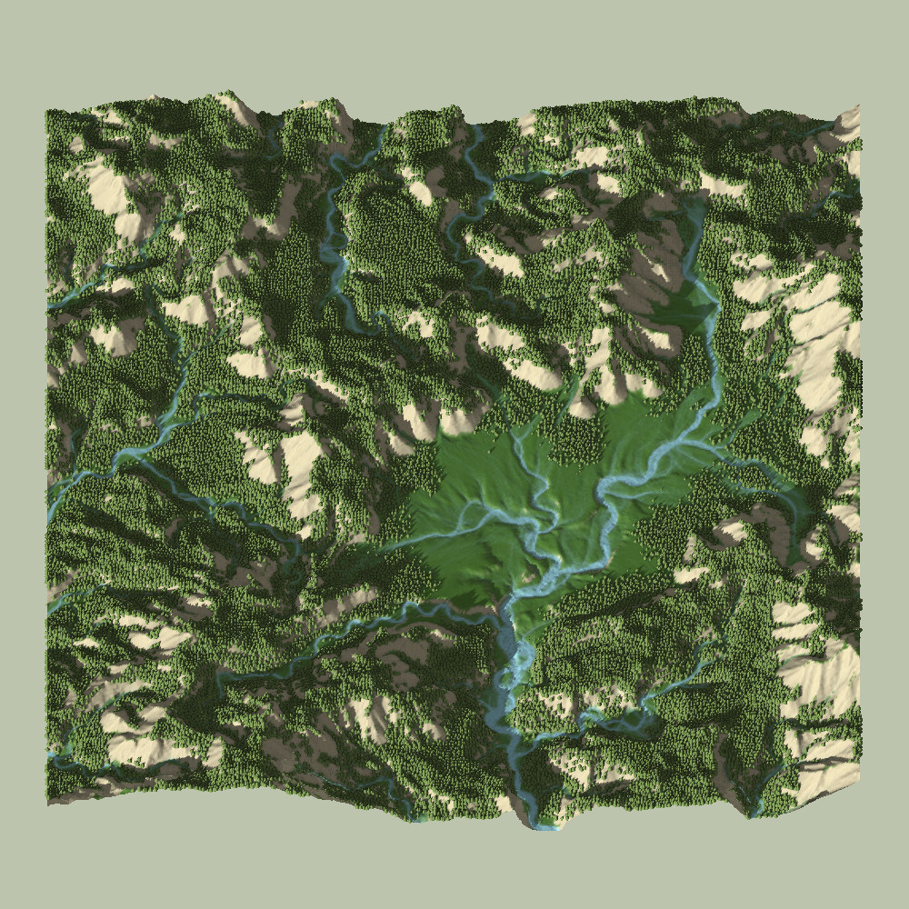
Results
Procedural Hydrology with Meandering
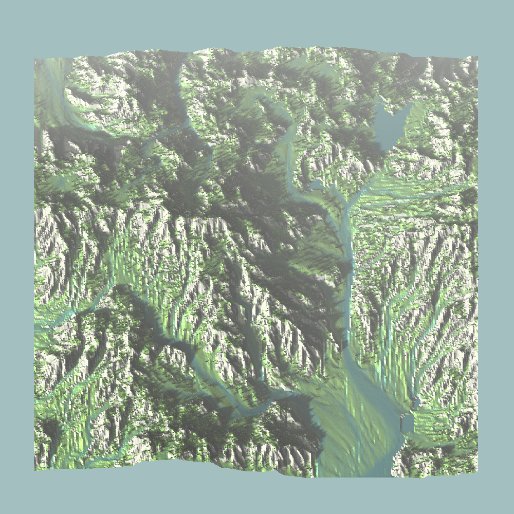
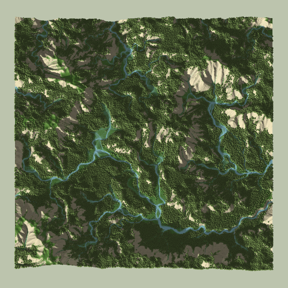
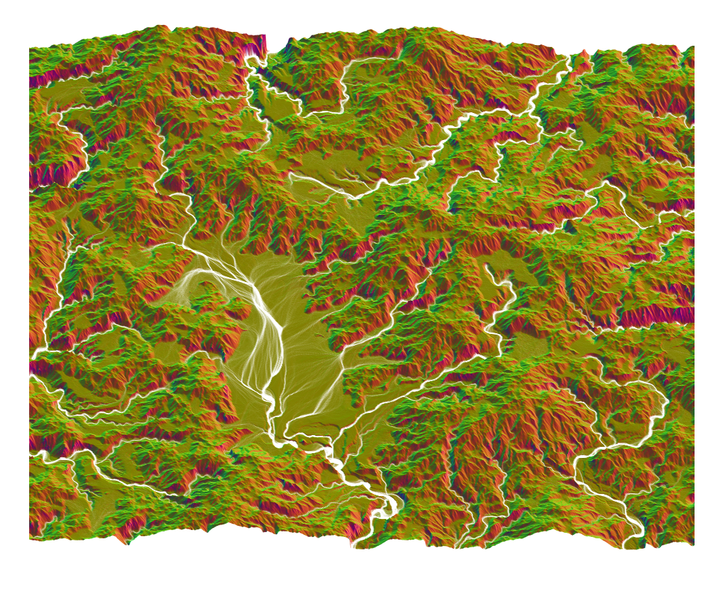
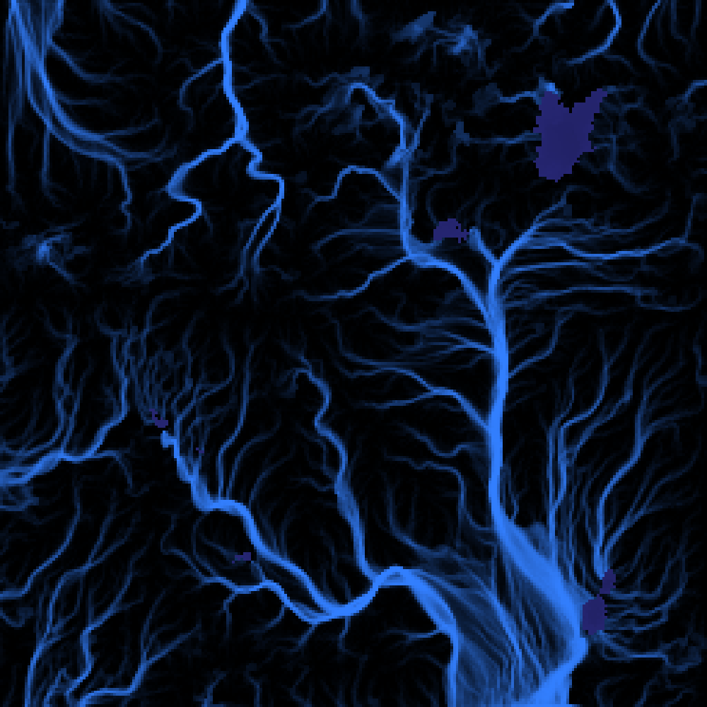
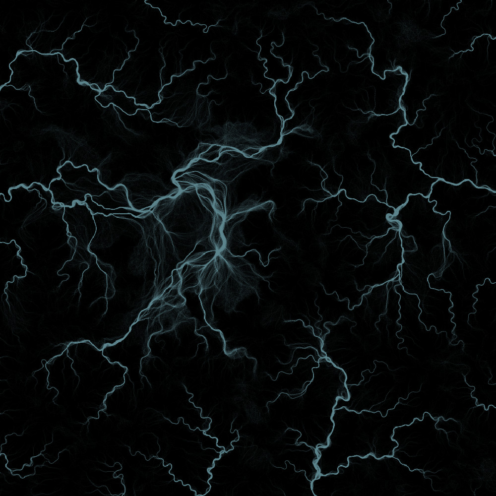
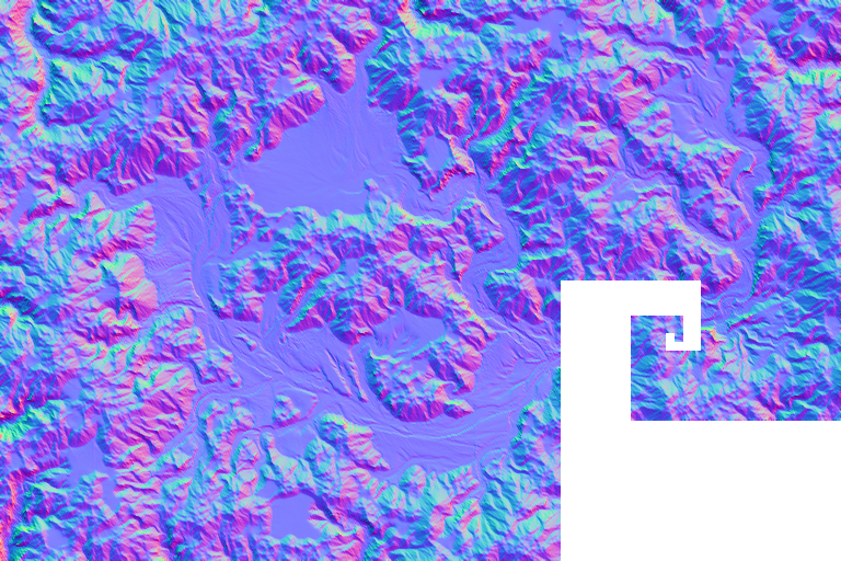
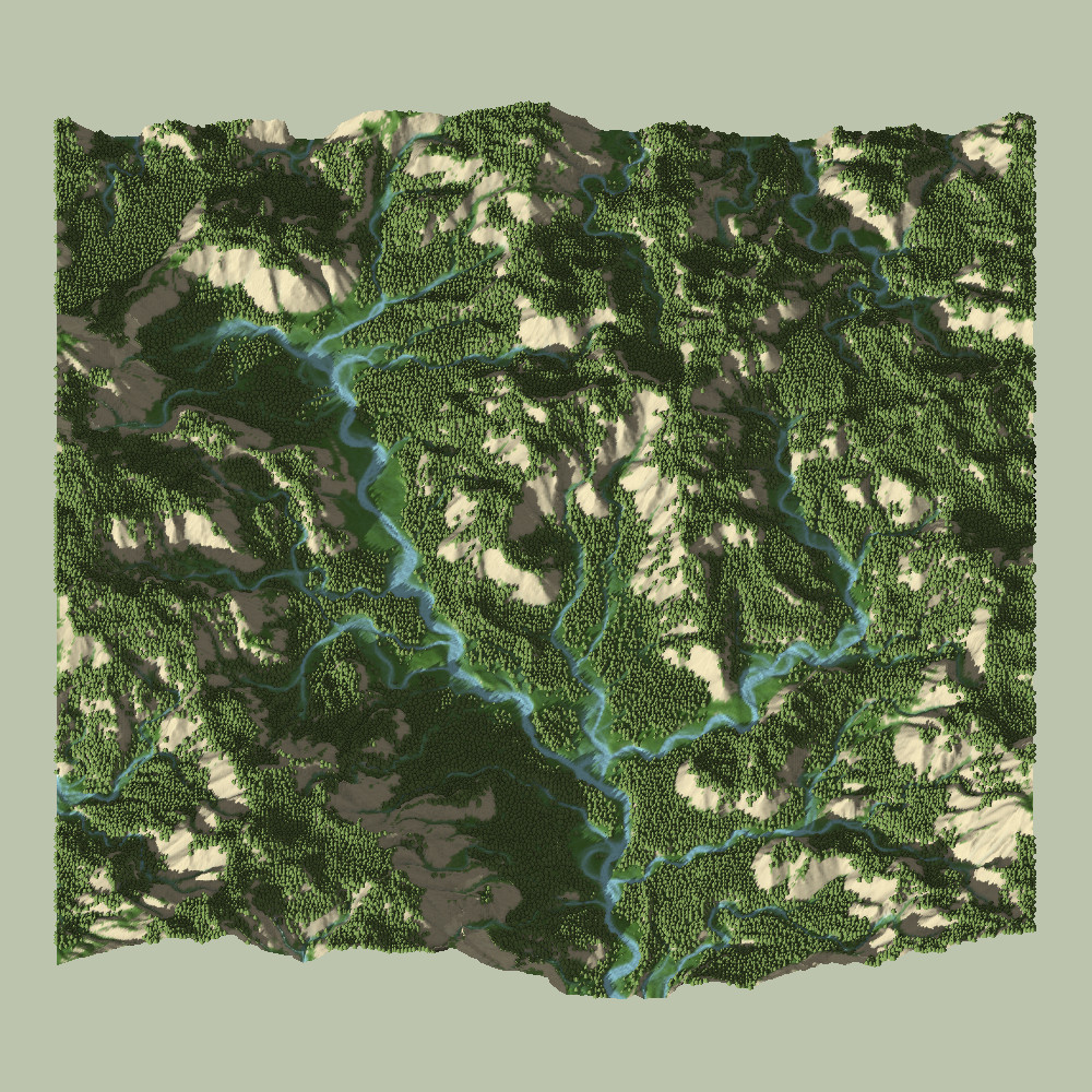
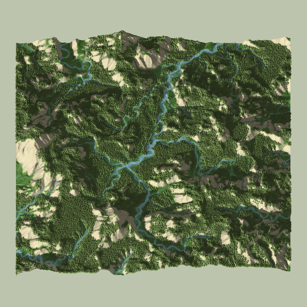
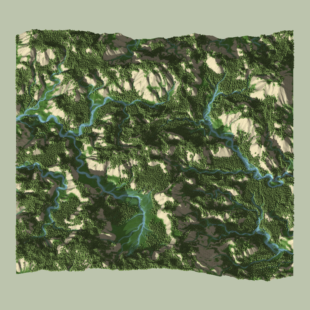
Overall, addressing all of the previously mentioned concerns helped the surface and stream maps increase in realism and detail. Here is a visualization of a 960×960 map’s surface and stream-map, after about 2000 time-steps:
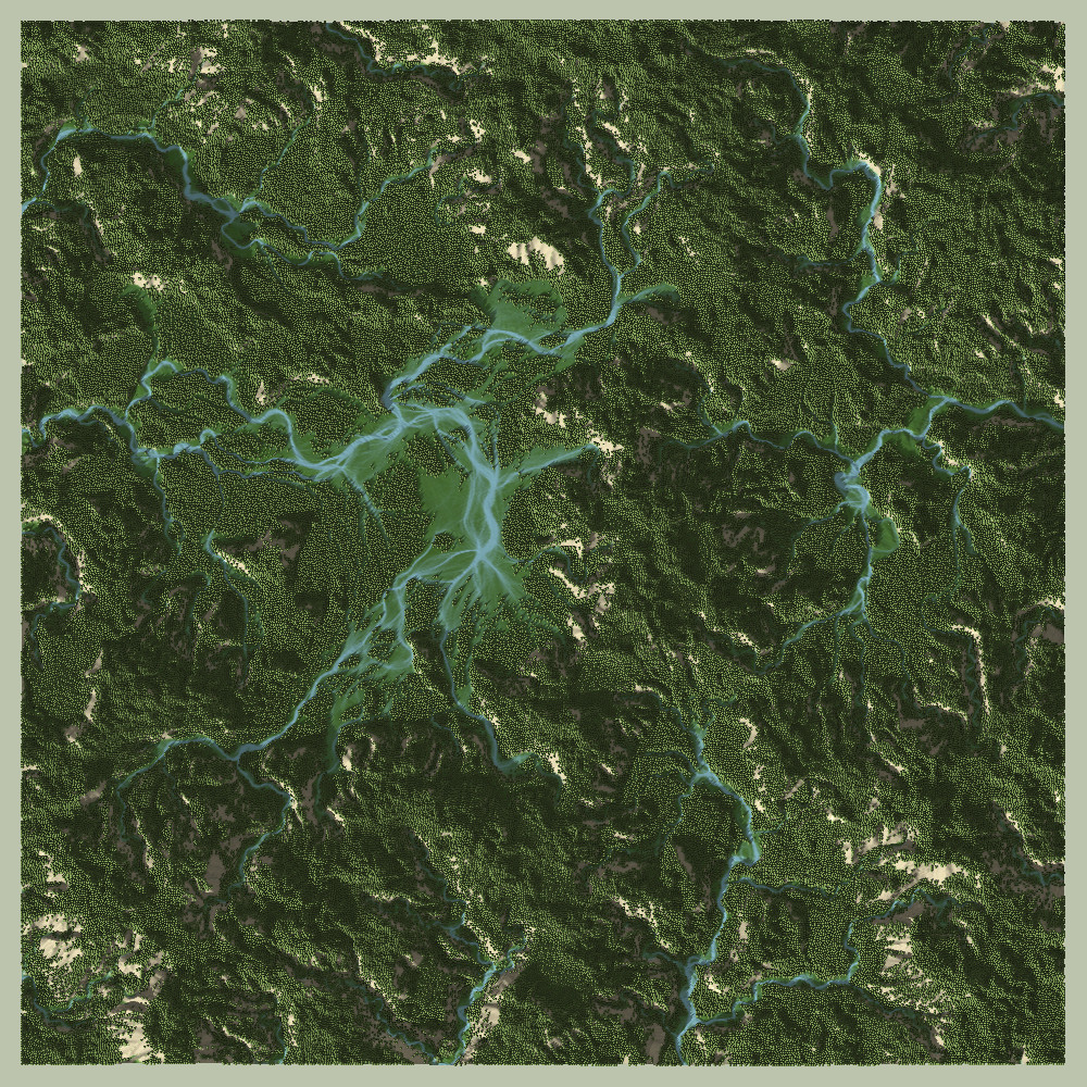
In all simulations, the initial terrain utilized is derived from fractal noise. This has the effect that the map doesn’t start with a valid water-shed due to many small and large basins.
Instead of filling these as an initial condition or allowing the basins to be filled with lakes (I deactivated those, remember?), I let the erosion simulation solve the basin problem. This divides the simulation into two phases: before and after the water-shed becomes valid.
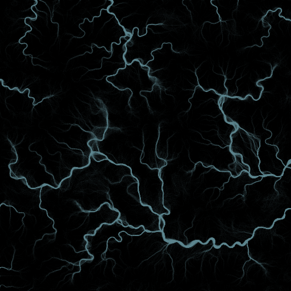
Here is an animation of streams solving the water-shed.
In the phase before the water-shed has been solved, we can observe ribbons and loops of streams circling the border of their basin in an attempt to break out and join other streams on their merry way downhill. In a way, the momentum conservation has implemented a water-shed search algorithm. That’s cool.
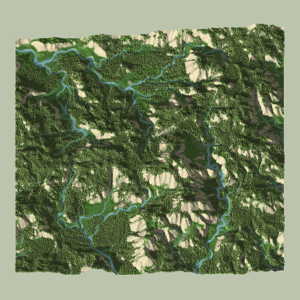
After the water-shed has been solved, we can easily visually verify that they streams are, in fact, meandering. Some tell-tale signs include:
- Steady Increase of Curvature on the Outer-Bank
- Slow Forward-Propagation of the Meander Curve
- Stream Cut-Off Behavior and Pinching
- Oxbow Lakes (which subsequently fade away)
- Meander Scarring (visible on surface maps)
The introduction of momentum conservation had another effect besides the meandering of streams: Streams are now more stable across longer distances, meaning that the simulation of larger maps becomes possible, with a caveat: Larger maps mean larger basins, and longer time to solve the basin problem before a larger water-shed forms.
Although I have not tried in earnest, I think that this is another necessary step towards simulating canyons. Now I just have to integrate this with multi-layer erosion!
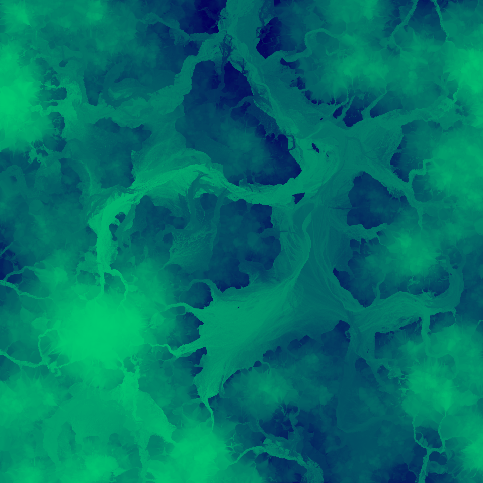
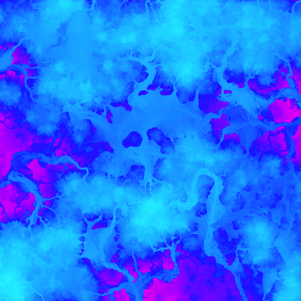
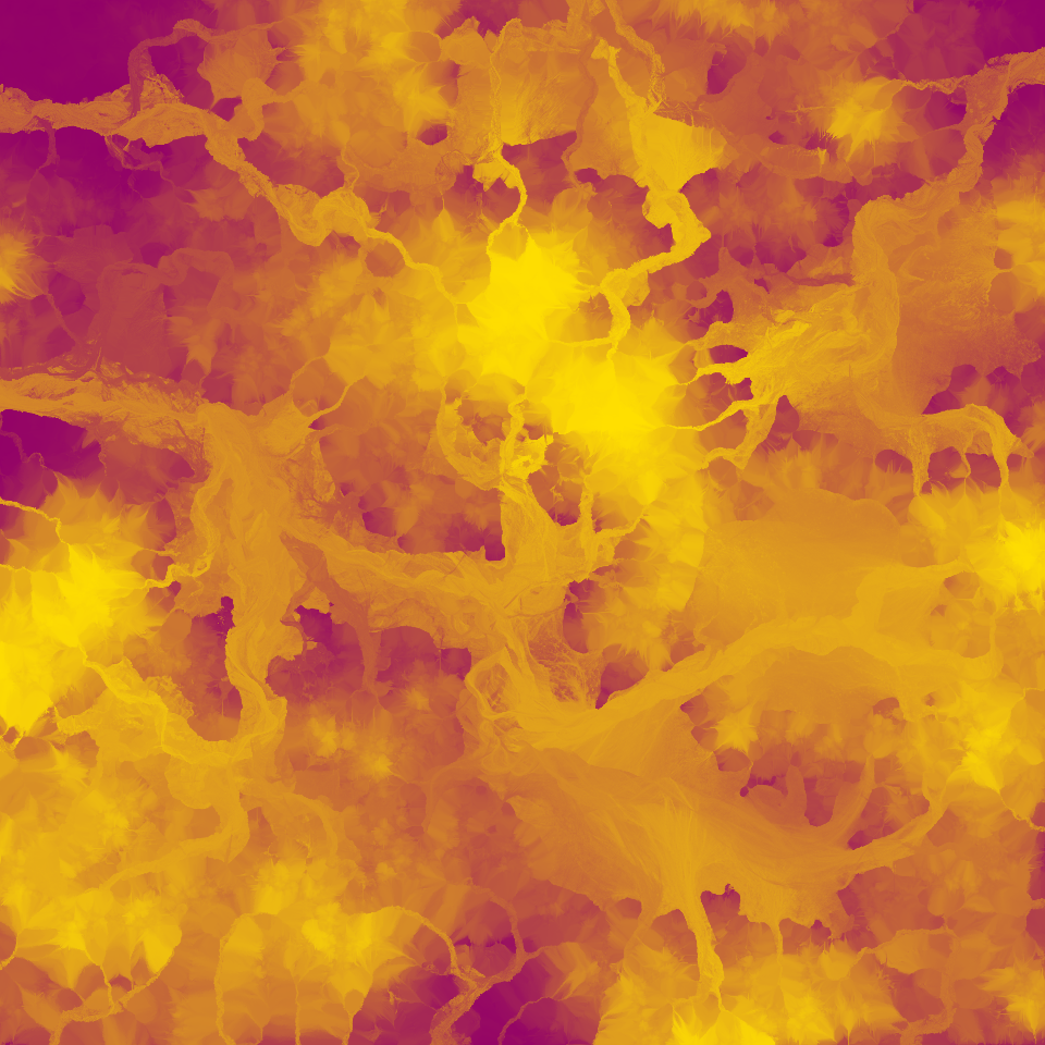
Meander Pigment Washing
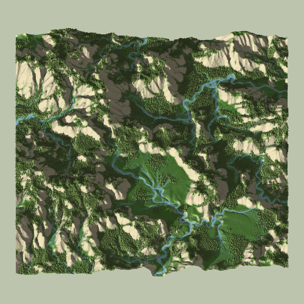
Trying to come up with a cool way to visualize the historic path of meandering rivers, I decided to model a map which contains a light soil (pigment) at high elevations with a linear gradient towards a dark soil (pigment) at lower elevations.
When picking up or dropping sediment, the two values would be mixed and thus dragged across the map in the path of the streams, and effectively visualize the historic path of the meandering streams.
That results in these cool visuals. Enjoy!
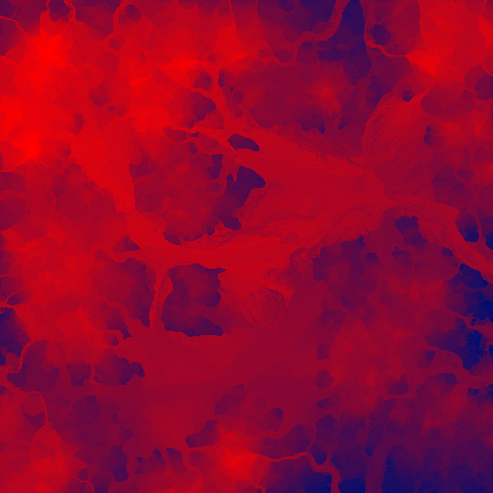
Note: The source-code for these visualizations is here.
Final Words
If you have read this far, thank you!
While meandering has been on the main branch of SimpleHydrology for quite a while now, it has taken me quite a bit of time to write this article. Not only for time reasons, but also because of my own standard of quality.
Originally, I wanted to also fix lakes definitively, but realized after months of toil that the scope was completely blown up. Not just because lakes are much more complex than I thought, but because there is already enough information for a full article after discussing the improvements to Procedural Hydrology over the years, which until now, have been undocumented besides the occasional reddit post.
With the amount of geomorphological simulation code I have written over the years, it is becoming increasingly difficult to manage and integrate into existing projects. For instance, when will SoilMachine support meandering? Should it? How much longer should SimpleHydrology be maintained into the future?
Attempting to integrate these changes into all these separate repositories probably doesn’t make sense at some point, and they might be archived at some point.
It is for that reason that I decided to unify these concepts in a C++ library called soillib, to allow me to base simulation implementations off of. Most of my most recent geomorphology code, including tools and other utilities, is now located there and will be updated there for the foreseeable future.
The goal is not only to unify the implementations, but offer convenient interfaces to perform geomorphological simulations on data, without the visualization. Tools include .tiff based pure command-line tools, for instance for generating a relief-shaded height-map:
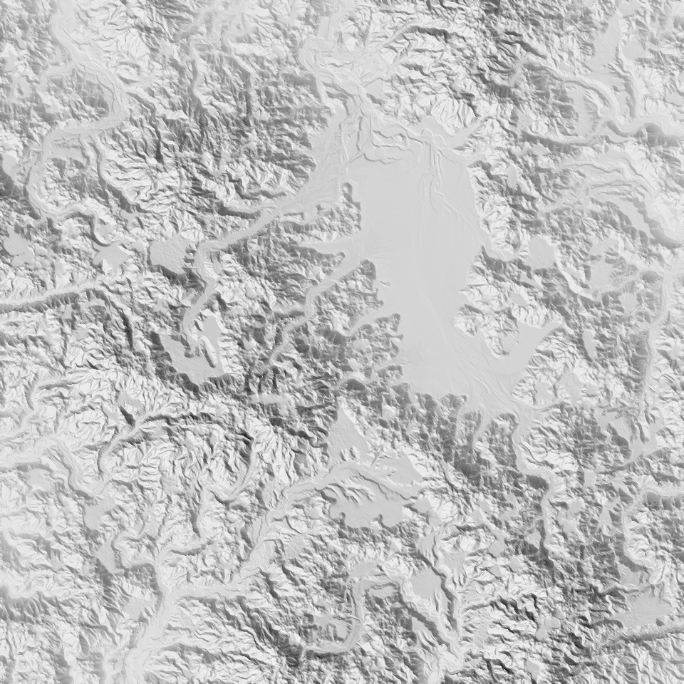
Additionally, it gives me a place to experiment with modularity and composition of various components, e.g. non-square maps to let the particles operate on.
Overall, I am quite happy with the results of the meandering.
In terms of outlook, the last thing I absolutely have to tackle before considering these projects “done” in any way is oceans and particularly shores and beaches. That would let me close off an island of a finite size to run the simulation on, and would make for a plausible, finite map. Everything else would just be for additional detail.
If anything in this article is unclear, you have any questions, or you are interested in collaborating on developing geomorphological simulations, feel free to reach out!
