Exploring the Iterative Circumcenter Map: GPU Acceleration

Note: This is a companion article to the publication Nicholas McDonald, Ronaldo Garcia, Dan Reznik, “Exploring the Dynamics of the Circumcenter Map”, Mathematical Intelligencer, 2022 (to appear). arXiv: 2202.02551

Around new year 2020/2021, I was contacted by Dan Reznik to see if I could help with generating some visuals for an interesting, novel mathematical system he had discovered and was analyzing together with Ronaldo Garcia. At the time, he had already published a related article on Wolfram.

The system in question is the “Iterative Circumcenter Map“, which exhibits very interesting dynamics in the plane using only basic principles from triangle-related geometry.

The iteration of the circumcenter map exhibits a spiral formed out of repeating triangle shapes. What this means and how this relates to the title image is explained further below.

Dan had described the problem as “embarrassingly parallel”, and I agreed, but he lacked the experience to properly GPU accelerate the computations and generate appropriate visualizations. I was intrigued and had some time on my hands, so I was happy to provide “computational support”.

The resulting collaboration ended up being a fun project in which I could flex my shader skills while contributing to mathematics in an area (triangle geometry) where it is difficult to open new avenues for research.

The GPU acceleration of the computation could generate the same images in microseconds which had previously taken him hours.

In the following article, I will define the system and describe how GPU acceleration was used to generate visualizations and provide insight which would have otherwise been infeasible.

The entire code used to generate these visualizations was written in C++ and is available, open source, on my Github. I am also working on an interactive WebGL version of the system so you can play around with it yourself!

Note: You can find the full source code for the C++ version of the GPU accelerated implementation of this system on my Github profile here. The relevant code sections are described below. This article and the repository will be updated when the WebGL version is completed.

The Iterative Circumcenter Map

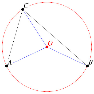
The circumcenter of a triangle is defined as the center of the triangle’s circumcircle. For a given triangle T=ABC, the circumcenter O(T) is unique. Note that equivalently, the circumcenter O is equal distance from the points A, B, C.

Note: The circumcenter is only one of many “triangle centers“, which are unique points that are invariant under given similarity transformations. Other examples include the centroid, incenter or orthocenter.

Using the circumcenter, we can now play the following game:

Define an additional, arbitrary point in the plane M
Define three new triangles MBC, AMC and ABM
Compute the circumcenter O(T) for each new triangle, defining A’=O(MBC), B’=O(AMC), C’=O(ABM)
The triangle T’=A’B’C’ is the next iteration of T given M

This process can then be repeated to yield iterations of T, based on an initial triangle T=ABC and an arbitrary point M.

The “anchor” point M is indicated by the red circle. Subsequent circumcenter map triangles are shown in this animation.

Note: This process is not only well-defined for triangles but for any given N-gon, as the vertices of the N-gon have a defined ordering. For a given N-gon P and point M, by maintaining the vertex ordering for the circumcenters in the next iteration, we receive another N-gon. Subsequently, we will only observe this more general case.

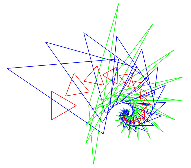
Dynamics of the Circumcenter Iteration

By iterating the circumcenter map, we make an observation:

For a given N-gon and point M, after N-iterations of the circumcenter map, we receive a similar polygon.

N iterations of the circumcenter map therefore represent a similarity transform in the plane. This similarity transform exhibits a rotation and scaling around M with constant scaling and rotation factors as the iteration progresses. As these factors are both constant, they naturally form a spiral.

Note that every polygon in the iteration can be considered its own initial condition, so the polygons cycle through a sequence of N “canonical” shapes.

A similar set of circumcenter map iterations for a non-convex 4-gon.

Note: And we have no idea why! But it’s pretty cool though.

Depending on the position of M relative to the polygon P, the degree of rotation and the scaling factor vary.

We observe that the scaling factor is bound between a lower bound (fastest possible shrinking rate) and infinity, i.e.:

(1) $\begin{equation*} 0 < s_{min} < s < \infty \end{equation*}$

Therefore, depending on the position of M relative to the original polygon, we observe either a converging or diverging spiral sequence of polygons around M.

We currently don’t know how to derive these similarity transform parameters, but we can compute them!

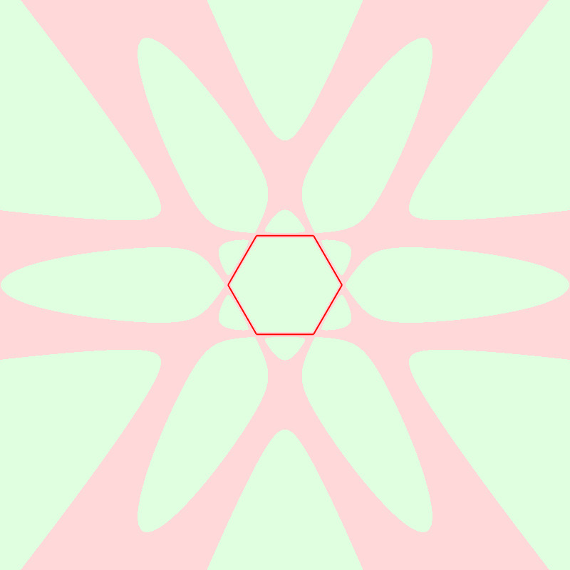
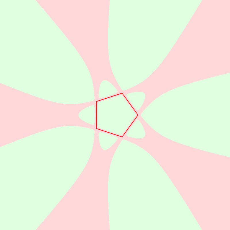
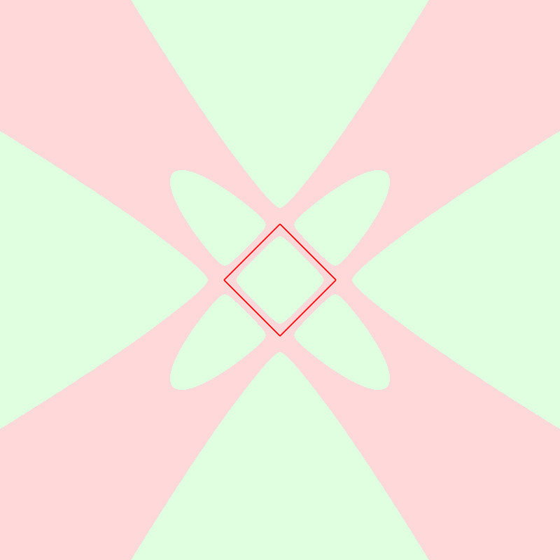
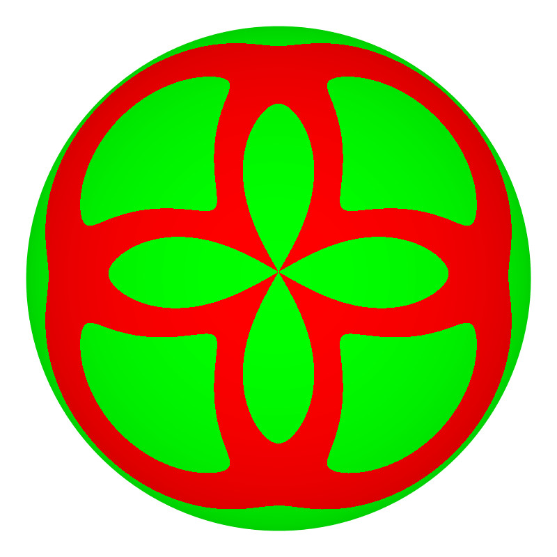
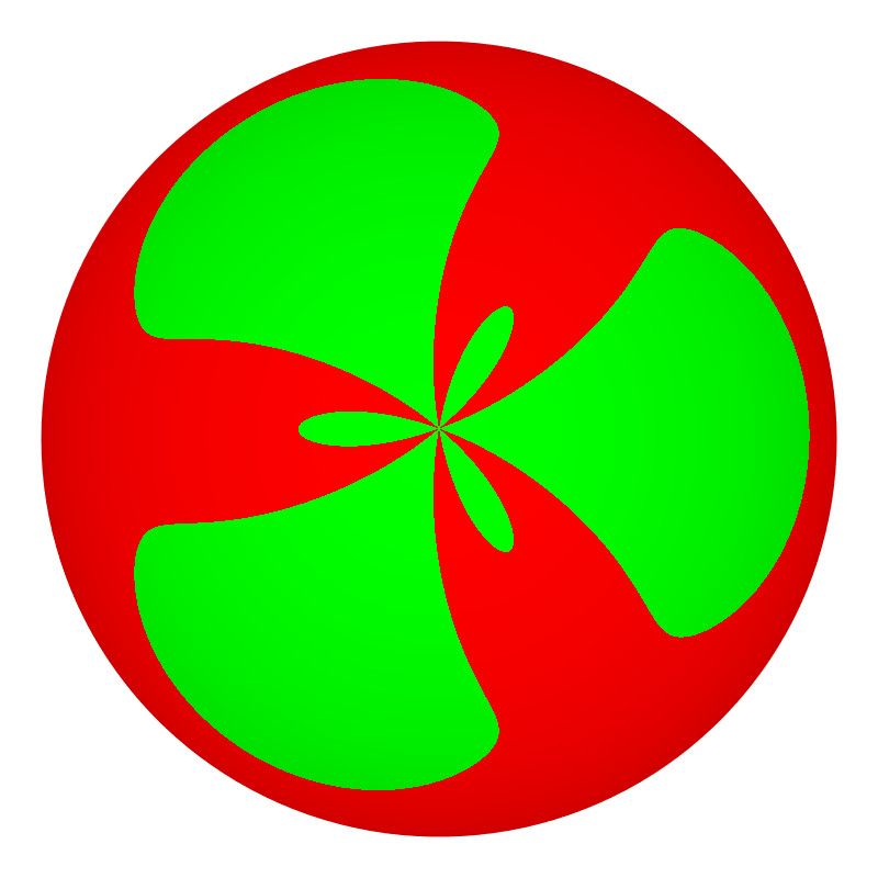
The Similarity Transformation Image

Placing some original polygon P in the plane, we can now determine the scaling factor for every possible M.

We can color the plane by determining whether the scaling factor s is smaller or larger than 1 (i.e.: convergent or divergent, constant on boundary) for M at the given position.

This yields the following images for N=3 to N=7:

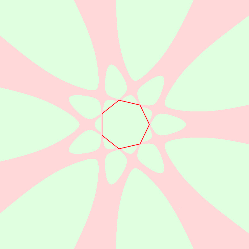
Similarly, we can use an HSL representation of the rotation to color the plane by the degree of rotation dependent on M.

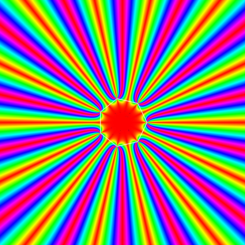
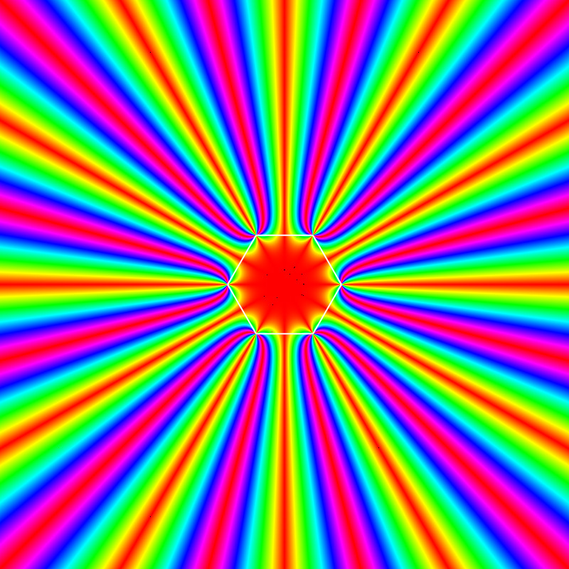
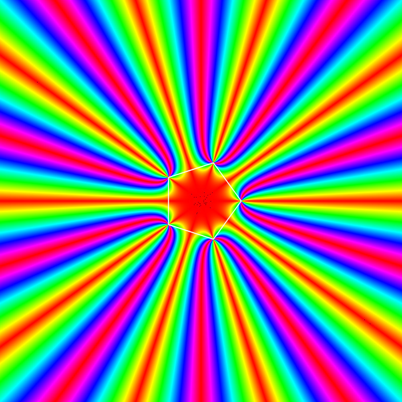
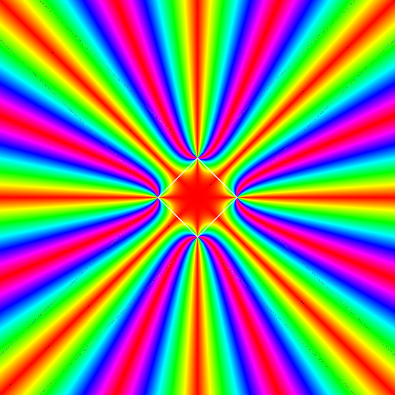
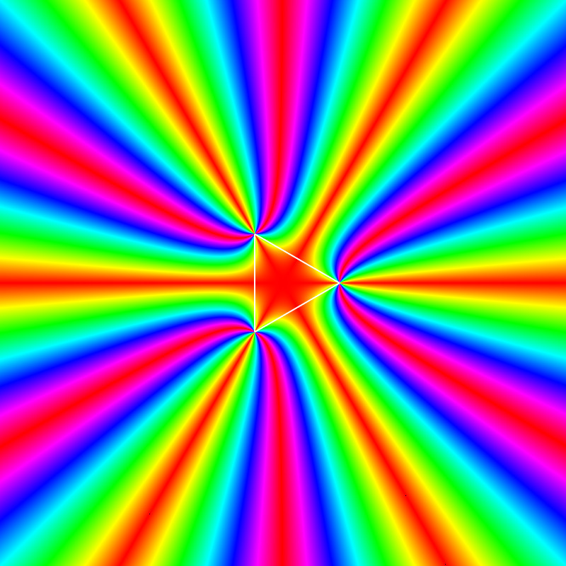
Note: These images are for the first 5 regular polygons, but the principle holds for non-regular and even non-convex polygons. For the rotation, the color red represents the invariant lines.

To generate these images, the circumcenter iteration needs to be repeated for N iterations on N vertices, for every pixel.

While these images are useful for analyzing the dynamics of the system, sequential computation on the CPU is naturally very slow and non-interactive. This is the problem I tackle in the remainder of this article.

The GPU Acceleration

In his own words, Dan described the problem of computing the image as “embarrassingly parallel“, and I agreed. I had some free time on my hands and was intrigued by the problem, so within the hour, I had a working prototype. The generated visualizations are fast enough to be manipulated in real-time, so all visualizations in this article are real-time.

The natural idea is to use a fragment shader to perform N iterations over the N-gon for every pixel in parallel, and then extract the relevant information for the similarity transform.

There are of course many implementation details, primarily related to memory efficiency and stability considerations, which I will go into below.

My first goal was to find a stable, shader-based solution for computing the circumcenter of a triangle.

The Circumcenter as a Matrix Inversion

My first observation was that computing a triangle’s circumcenter could be expressed as a matrix inversion problem. This is extremely convenient and provides direct, intuitive insight into where and why stability issues arise.

We observe that the circumcenter O of a triangle T is equal distance r from all points A, B, C. Expressing all points as vectors, this condition can be written using the dot-product:

(2) $\begin{equation*} ( \underline{A} - \underline{O} )^T( \underline{A} - \underline{O} ) = r^2 \end{equation*}$

(3) $\begin{equation*} ( \underline{B} - \underline{O} )^T( \underline{B} - \underline{O} ) = r^2 \end{equation*}$

(4) $\begin{equation*} ( \underline{C} - \underline{O} )^T( \underline{C} - \underline{O} ) = r^2 \end{equation*}$

Note: In this notation O implies a column vector.

By expanding the dot-products, this is equivalent to:

(5) $\begin{equation*} \begin{aligned} \underline{A}^T\underline{A} - 2\underline{A}^T\underline{O} & = \\ \underline{B}^T\underline{B} - 2\underline{B}^T\underline{O} & = \\ \underline{C}^T\underline{C} - 2\underline{C}^T\underline{O} & \end{aligned} \end{equation*}$

Which can be re-expressed in the two equations:

(6) $\begin{equation*} ( \underline{B} - \underline{A} )^T\underline{O} = \frac{1}{2} (\underline{B}^T\underline{B} - \underline{A}^T\underline{A}) \end{equation*}$

(7) $\begin{equation*} ( \underline{C} - \underline{A} )^T\underline{O} = \frac{1}{2} (\underline{C}^T\underline{C} - \underline{A}^T\underline{A}) \end{equation*}$

Note that by stacking these two equations, we can finally express our circumcenter as a linear system of equations, solved by inverting a matrix:

(8) $\begin{equation*} \underline{O} = \frac{1}{2} \begin{bmatrix} ( \underline{B} - \underline{A} )^T\\ ( \underline{C} - \underline{A} )^T \end{bmatrix}^{-1} \begin{bmatrix} \underline{B}^T\underline{B} - \underline{A}^T\underline{A}\\ \underline{C}^T\underline{C} - \underline{A}^T\underline{A} \end{bmatrix} \end{equation*}$

Note: I have never seen a derivation of the circumcenter in this manner before online. Please let me know if you have a reference. Other references I found either solve a line-intersection problem (which is mathematically related), or using a complicated series of conditionals.

Computational Stability

Based on the matrix-inversion formulation of the problem, determining stability of the computation becomes relatively simple: The computation diverges when the determinant of the matrix approaches zero, i.e. the matrix is singular.

This is a convenient check that is exploited in the shader.

Note: This condition is given when all points in the triangle become co-linear, which can be seen intuitively by the matrix determinant becoming zero – i.e. the vectors BA and CA are co-linear.

General Triangle Centers by Matrix Inversion

Similar to the circumcenter, an analogous linear system of equations can be derived for other triangle centers.

For instance, the orthocenter is given by:

(9) $\begin{equation*} \underline{H} = \begin{bmatrix} ( \underline{B} - \underline{A} )^T\\ ( \underline{C} - \underline{A} )^T \end{bmatrix}^{-1} \begin{bmatrix} \underline{B}^T\underline{C} - \underline{C}^T\underline{A}\\ \underline{C}^T\underline{B} - \underline{B}^T\underline{A} \end{bmatrix} \end{equation*}$

Note that the inverted matrix is identical, only the vector it is multiplied by is different. The derivation is left as an exercise to the reader (I have always wanted to write that!).

The Fragment Shader

Note: The vertex shader is not of primary interest, because it renders a full screen quad for use in the fragment shader, which is executed once for every fragment (in this case: screen-space pixels). The following section is written in GLSL code.

The fragment shader code is relatively brief. The core goal of the shader is to perform the circumcenter iteration and color the frame buffer based on computed scaling or rotation.

We start by providing the texture position, an output color, a number of vertices N and a shader storage buffer object (SSBO) that provides the 2D coordinates of the vertices.

#version 430 core

in vec2 ex_Tex;
out vec4 fragColor;

uniform int N;

layout (std430, binding = 0) buffer pointset {
  vec2 p[];
};

const float PI = 3.14159265f;

// Convergence / Divergence Colors
const vec3 diverge = vec3(1.0, 0.85, 0.85);
const vec3 converge = vec3(0.88, 1, 0.88);

// Interface Controls
uniform float zoom;
uniform vec2 center;

// ...

We implement the circumcenter computation function and stability checks based on our previous derivation:

//...

bool iscoplanar(vec2 M, vec2 A, vec2 B) {

  return abs(determinant(mat2(A.x-M.x, B.x-M.x, A.y-M.y, B.y-M.y))) < 1E-8;

}

vec2 circumcenter(vec2 M, vec2 A, vec2 B) {

  mat2 Q = inverse(mat2(A.x-M.x, B.x-M.x, A.y-M.y, B.y-M.y));

  return Q*0.5*vec2(dot(A,A)-dot(M,M), dot(B,B)-dot(M,M));

}

// ...

Finally, in our main function we perform the iteration

void main(){

  // Position of this fragment (i.e.: local anchor point)
  
  vec2 M = (ex_Tex*2-vec2(1)+center)/zoom;

  // Ping-Pong Buffers (Copy)

  const int K = 32;
  vec2 tempsetA[K];
  vec2 tempsetB[K];

  for(int i = 0; i < N; i++){
    tempsetA[i] = p[i];
    tempsetB[i] = vec2(0);
  }

  //Check Co-Planarity

  for(int i = 0; i < N; i++){
    if(iscoplanar(M, tempsetA[i], tempsetA[(i+1)%N])){
      fragColor = vec4(diverge, 1.0);
      return;
    }
  }

  // Perform Iteration

  for(int i = 0; i < N; i++){   //Iterate N Times
    for(int k = 0; k < N; k++){ //Over N Intervals
      if(i%2 == 0) tempsetB[k] = circumcenter(M, tempsetA[k], tempsetA[(k+1)%N]);
      else tempsetA[k] = circumcenter(M, tempsetB[k], tempsetB[(k+1)%N]);
    }
  }

  // Compute the Scale Factor

  float scale = 1.0;
  if(N%2 == 0) scale = length(tempsetA[1] tempsetA[0])/length(p[1]-p[0]);
  else scale = length(tempsetB[1]-tempsetB[0])/length(p[1]-p[0]);

  // Set the Color

  if(scale < 1) scale = 0;
  else scale = 1;
  fragColor = mix(vec4(converge,1), vec4(diverge, 1), scale);

}

A similar method can then be used to color based on rotation, e.g. using HSL transformation and visualizing hue.

Note: GLSL shaders don’t allow for dynamic arrays. We allocate two ping-pong buffers of K = 32 possible vertices that each fragment shader computation instance uses. This implicitly limits us to a polygon of 32 vertices, but at that point the program becomes prohibitively slow anyway.

Implementation Details

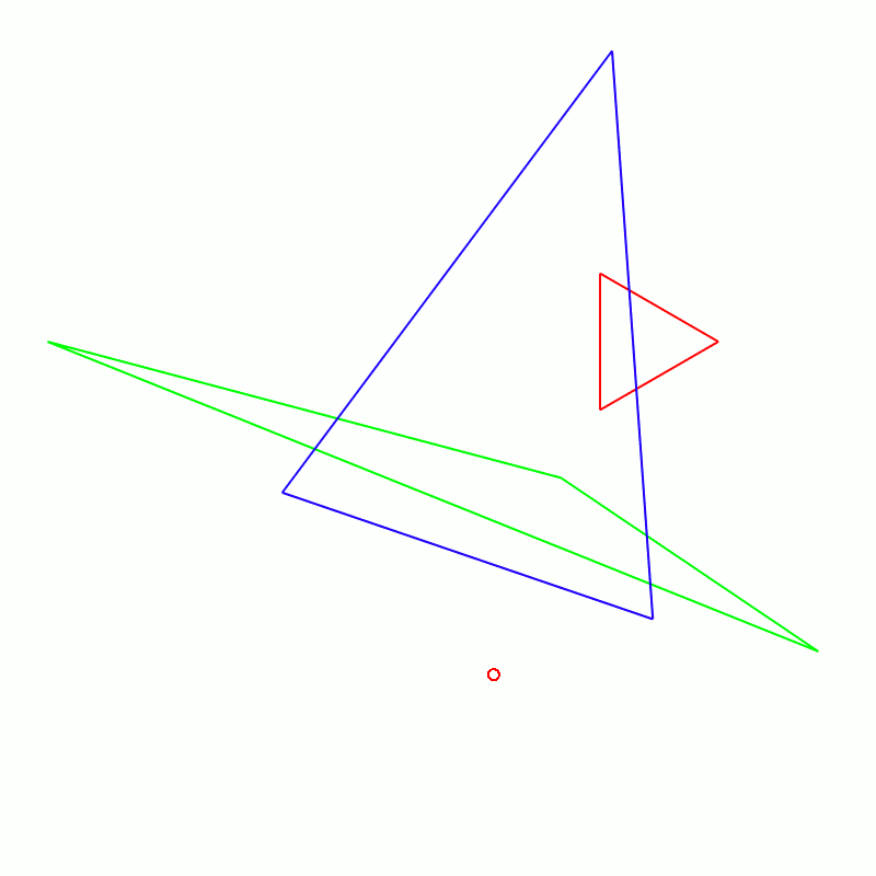
By adding an interactive way to modify the SSBO from the CPU, the simulation becomes fully interactive and we can observe how the iterative circumcenter map changes as vertex positions are altered.

A real-time animation of the interactive circumcenter map program. A single frame of this video previously took hours to compute.

Additional Visualizations

Stereographic Projection

Dan had the idea to utilize a stereographic projection to see what happens as M moves infinitely away from the polygon.

The stereographic projection maps all points on a sphere to the plane, but can also be used for the inverse operation.

For a given point on the unit sphere p = (x, y, z), where |p| = 1, we can compute a point on the plane P = (X, Y) using:

(10) $\begin{equation*} (X, Y) = k (\frac{x}{1-y}, \frac{z}{1-y}) \end{equation*}$

where k is some scaling factor and y is the coordinate orthogonal to the plane.

Points which are infinitely far from the plane’s origin:

(11) $\begin{equation*} (X, Y) \to \infty \end{equation*}$

are thus conveniently mapped to the sphere’s “north pole”, which allows us to analyze behavior at the planes extrema.

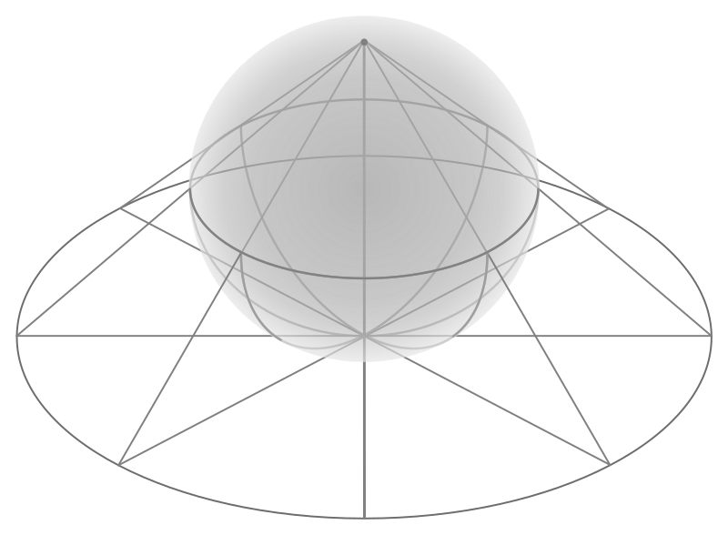
Note: Here we see stereographic projections of the scaling factor stability region images, viewed from the north pole.

To generate these visualizations, we mesh an icosphere by recursively sub-dividing the triangle faces of an icosahedron into 4 smaller triangle faces and normalizing the vertices.

The rendering pipeline then projects the faces into screen-space, rasterizes them and provides the fragment shader with a convenient 3D coordinate, which we can normalize and use to sample the stability behavior of our plane, with the resolution exactly matching our screen resolution!

Note: Technically, any geodesic polyhedron is sufficient, but an icosphere is the easiest to mesh. Here is the code for it.

This is also fast enough for full interactivity.

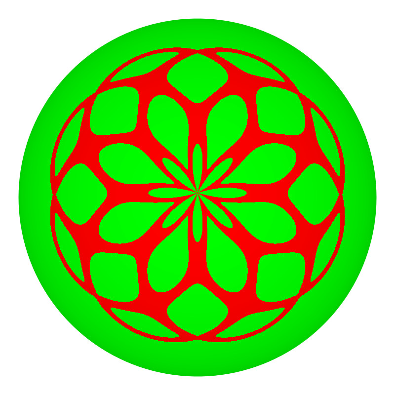
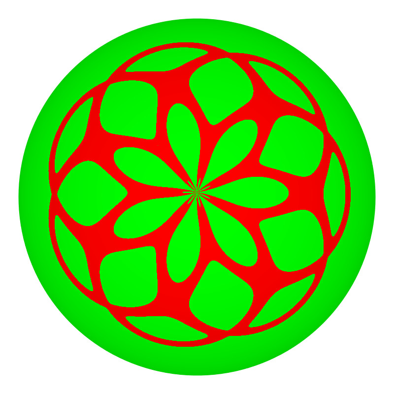
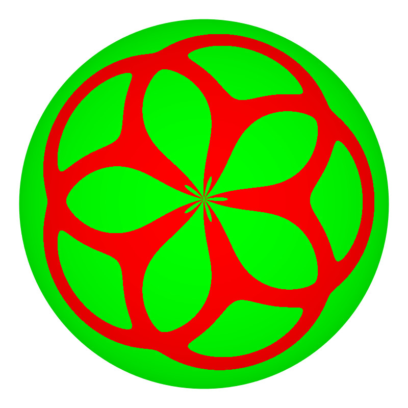
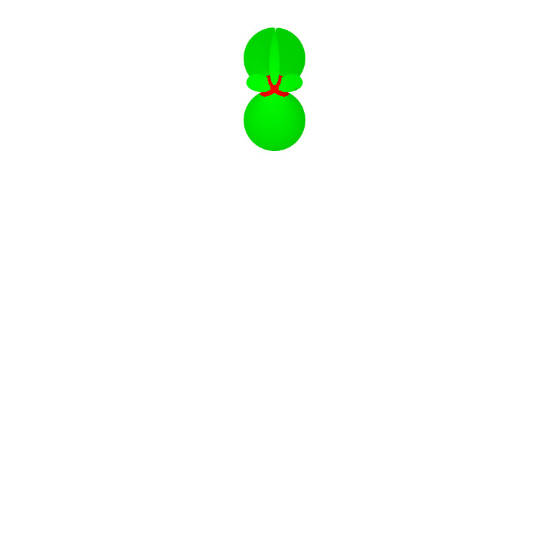
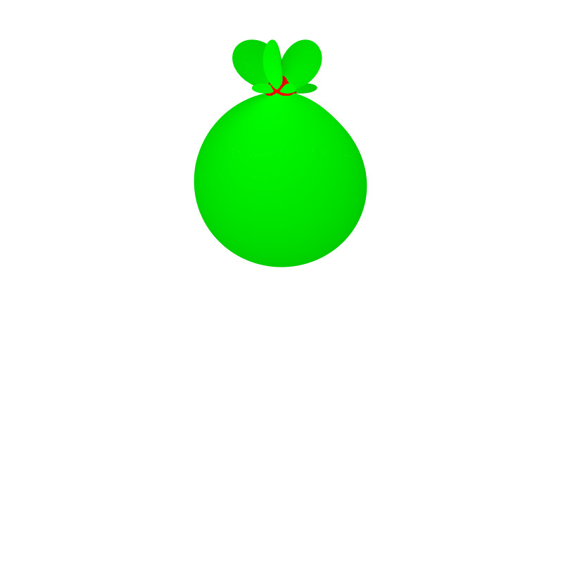
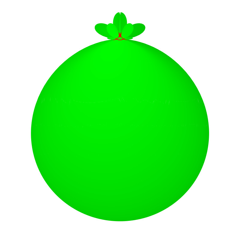
We can also effectively visualize the degree of scaling in 3D using our very first observation, namely that the scaling factor has a lower bound larger than zero and an upper bound at infinity.

Using a high resolution icosphere, we scale each vertex by the inverse of the scaling factor sampled from the plane.

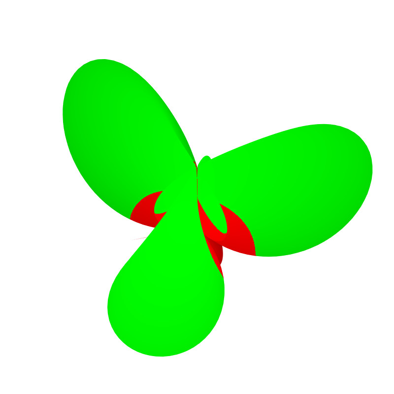
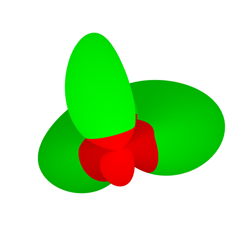
Note: This is the shape shown in the animation of the title image, shown here from three angles – top, side and bottom. Note that the circumcenter iteration sampled from the plane is for an equilateral triangle centered on the origin. The shape strongly resembles orbitals known from quantum mechanics.

The boundary between the red and green regions of course lies on the unit sphere, while the extrema of the green regions represent the fastest convergence, and infinite growth (i.e.: co-linearity) is mapped to the origin.

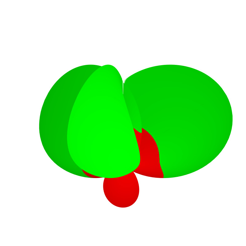
Finally, here are the same scaled projections for other origin-centered regular polygons, with relative scale preserved.

We note that the rate of convergence for most of the separated regions remains relatively constant while a single region at the south pole, i.e. in the center of the polygon, has a convergence rate which grows as N increases.

Ray-marched Sweep-Hull

The final interesting visualization we could think to come up with was to generate a sweep hull of the stability regions as the original triangle undergoes a parameterized transformation, for instance an affine transform.

An animated sweep-hull of an equilateral triangle undergoing an affine transform. Here, we are visualizing the divergent regions. This is a real time animation.

This is a challenging problem which I was glad to tackle. In keeping with computing the circumcenter iterations only on the GPU, my idea was to apply the method of ray-marching.

In a nutshell, this method works by emitting a ray for each pixel on screen and computing the shape intersection.

Note: To do this, we simply render a quad to the frame buffer in the vertex shader and emit the rays in the fragment shader.

This typically requires a signed-distance field, which assigns a distance d to the surface to every point in space (x,y,z).

As the ray knows its distance from the surface, it can “march” forward by that distance iteratively, and the surface is intersected if the distance drops below a threshold value.

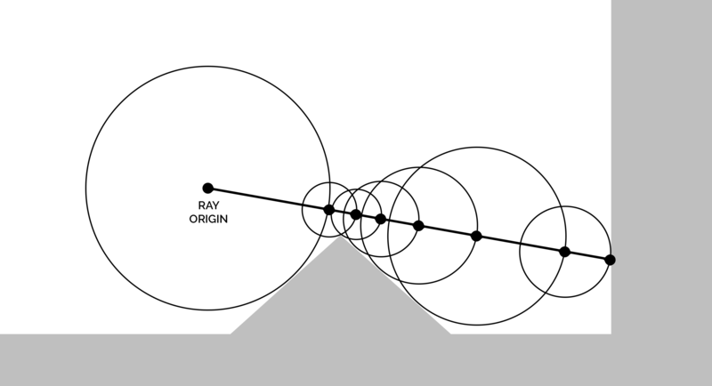
Wikimedia Commons, Visualization of SDF ray marching algorithm, Teadrinker

While the iterative circumcenter map does not provide a signed-distance field to the stability boundary, we can approximate one by taking the logarithm of the scale factor.

This has the effect that the boundary with scaling factor 1 is mapped to 0, while the convergent and divergent regions boundaries are mapped to negative and positive distance values respectively.

This also means that the inverse of the sweep hull is easily computed by taking the inverse sign of the log scale.

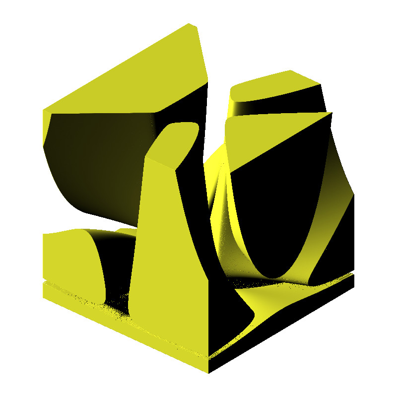
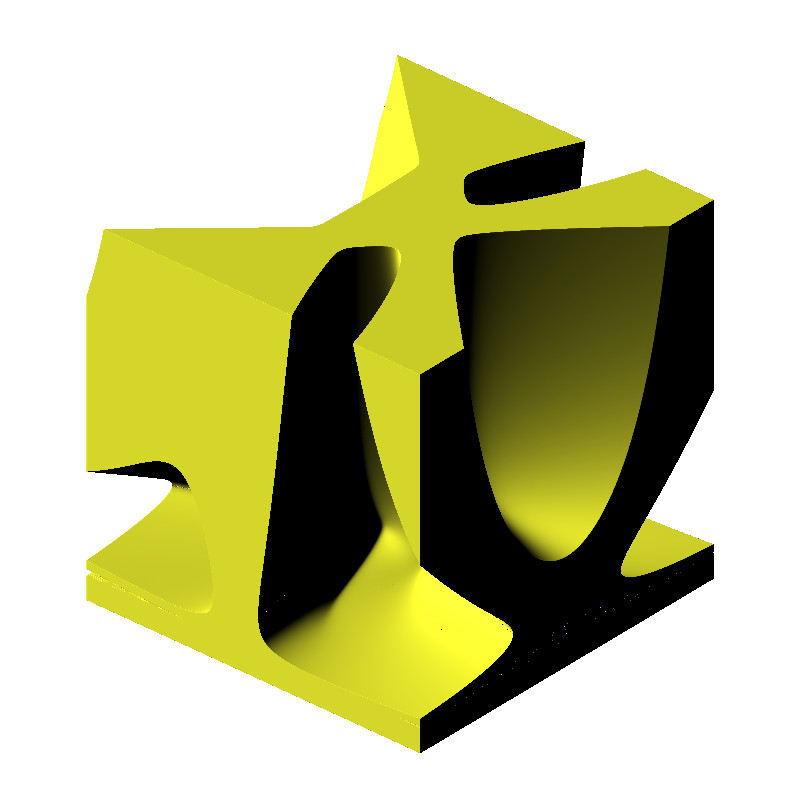
Note: Stability can be enhanced at the cost of more marching steps by only stepping a fraction of the estimated distance. For these visualizations, I used a stepping factor of 0.1. Still, some noise can be seen as is common with ray-based methods. The shading method can be found in the fragment shader code, but is essentially normal estimation by super-sampling

Visualizing Isolines and Stable Points

Since we are describing a convergent and a divergent region for the scaling factor of the iterative circumcenter map, it is desirable to visualize their boundary directly.

This is challenging, because we only have a texture with both regions and no explicit form for the boundary to e.g. trace it.

Generally the visualization of isolines is a tricky subject.

A naive approach would be to define a fragment as “on the boundary” if the distance of its scale from the isovalue drops below a certain fixed threshold. The problem with this approach is glaringly obvious once implemented:

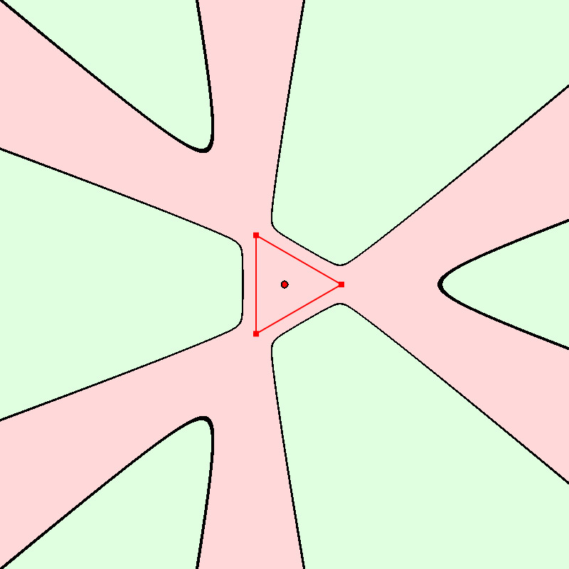
We observe that the isoline has varying thickness along the boundary, due to the gradient of the scaling factor.

It is in my opinion not only hard to find a good threshold, but impossible, and this approach should be abandoned.

The alternative is to generate the isolines in two-passes:

Generating the region texture without the isoline
Sample the texture with a 2×2 kernel to determine the boundary in analogy to a dilation kernel.

This guarantees that the isoline has constant thickness in screen-space, yielding an aesthetic line that is visually identical to an explicitly traced line at every scale.

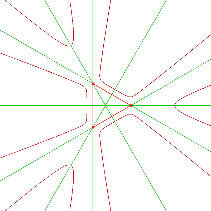
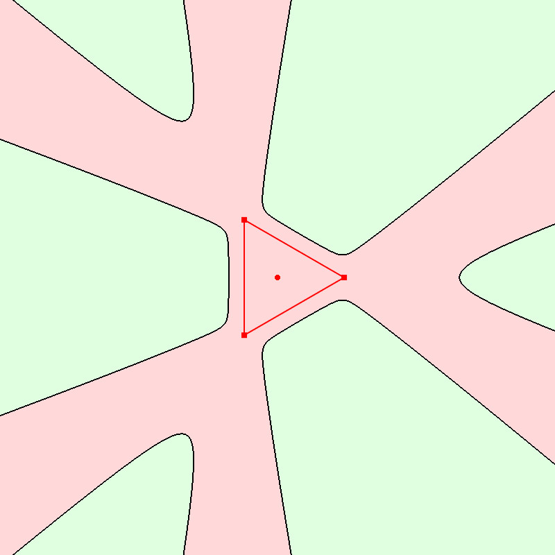
This can also be done for rotational invariant lines (above). Note that where these lines intersect, we have rotation and scale invariance, implying that the iterative circumcenter map cycles through not only a series of similar polygons but identical ones.

These “stable points” can exist for all discussed cases.

Note: A natural question that arises is: How many of these “stable points” exist for a given polygon geometry? No idea!

Final Words

While this article explores the implementation details for how various visualizations of a novel mathematical system were generated, the paper goes into more detail about the dynamics that it exhibits.

One interesting example is that stable points “inside” the polygons actually exhibit a double cycle (i.e. 2N steps) with rotational symmetry around the anchor point.

It appears that very little is still understood about this, so I’m glad to write this up and hope that it catches some attention.

I had a great time making these graphics and animations and hope you had a good time reading this and looking at them.

Thank you for making it this far!

If you are a mathematical researcher and need some help / advice on GPU acceleration of certain computational tasks or making pleasing visuals, I am happy to help. Feel free to reach out!