Note: The code for this article is available on my Github [here].

The other day I had an idea for how one can leverage the power of the GPU to generate voronoi textures.

The idea is to utilize an OpenGL depth test to perform conical intersections by writing the distance-to-centroid to the depth buffer in the fragment shader, with an instanced render.

It turns out this idea was not entirely new, but my idea is slightly different (and faster!), so I decided to implement it (using my TinyEngine) to see how performant it was.

Note: Key changes are a point distribution assumption for performance, a different approach to depth testing, dynamic centroid capabilities due to new OpenGL features (i.e. modern OpenGL) and implementation in C++ / general optimization.

I was positively surprised that it was very performant. In fact, it was so performant that generating voronoi diagrams
at over 60 FPS, for upwards of 2^16 nodes and an image of size 1024×1024 (with limitations!).

In this article, I will explain the general concept, implementation and some potential applications of real-time voronoi texture generation.

Voronoi Diagrams

A voronoi diagram is uniquely defined by a set of N points (“centroids”) in some space (in our case: 2D).

The diagram is an image where each pixel is colored by the index i of whatever centroid is nearest. The diagram is thereby essentially a clustering / labeling of pixels to centroids by a distance function.

The line between any two regions is the perpendicular bisector of their centroids’ connecting line. This is because positions on the boundary between two regions are equally far away from both centroids, or the value of the distance function to both centroids is equal.

If we picture a 3D plot where we plot the distance to the origin on the z-Axis for each position (x,y), we get a cone.

The separation lines between centroids thereby correspond to lines where the two centroids’ cones intersect (i.e. values are the same), projected onto the 2D plane.

As two cones intersect, one cone passes over the other, i.e. they change their “stacking order”. Looking at the combined intersections from below at a given point, only the lowest cone will be visible, which is the cone with its centroid nearest to that point.

Therefore, coloring all cones and performing a depth-test on their intersections from below yields the voronoi diagram. This concept is exploited on the GPU.

Generating Voronoi Diagrams

Given a set of centroids, the task is to either generate the edge and corner information or to generate a labeling image. These two representations are interchangeable for arbitrary resolution images.

Fast algorithms exist for generating the vertex data (such as Fortune’s Algorithm). Direct vertex data is necessary for certain applications, such as using these diagrams as a mesh or network structure.

For other applications it is sufficient to generate a voronoi texture. Such an approach lends itself well to generation on the GPU. My implementation is explained below.

GPU Accelerated Texture Approach

An OpenGL fragment shader will run a certain piece of code for every pixel on screen. Because a voronoi diagram is just a clustering, a simple naive implementation comes to mind:

1. Pass all centroids to shader in a buffer
2. Iterate over all centroids, find nearest index
3. Set pixel color based on index

Iteration over all centroids in the fragment shader is very slow, particularly when the image becomes large and a high number of centroids is used. This doesn’t scale well.

Instead, it is possible to utilize the built-in depth-test to perform the cone intersections that give the diagram:

1. Instance render a quad N times, passing centroid i
2. Color the entire quad uniformly according to i
3. Write the distance to centroid to the depth buffer

The resulting depth test then performs the intersection by only drawing the portion of all quads which are in the front. We then have our voronoi texture!

Implementation

Voronoi Shader

The voronoi texture is generated in a single shader program.

Vertex Shader

The vertex shader takes a full screen quad and an instanced centroid. Since the entire quad is one color, the color is computed in the vertex shader by converting gl_InstanceID into a color. The quad is scaled by R and shifted by the centroid (centroid is instance passed!).

#version 330 core
layout (location = 0) in vec2 in_Quad;
layout (location = 2) in vec2 in_Centroid;

out vec2 ex_Quad;
flat out vec3 ex_Color;
out vec2 ex_Centroid;

uniform float R;

vec3 color(int i){
  float r = ((i >>  0) & 0xff)/255.0f;
  float g = ((i >>  8) & 0xff)/255.0f;
  float b = ((i >> 16) & 0xff)/255.0f;
  return vec3(r,g,b);
}

void main(){
  ex_Centroid = in_Centroid;         //Pass Centroid Along
  ex_Color = color(gl_InstanceID);   //Compute Color
  ex_Quad =  R*in_Quad+in_Centroid;  //Shift and Scale
  gl_Position = vec4(ex_Quad, 0.0, 1.0);
}

The quad could theoretically be translated and scaled by a model matrix, by passing a 4×4 float matrix per instance.

Since all regions are drawn as quads with a fixed size (given by the expected particle inter-distance), it is cheaper to pass 2 floats per instance (i.e. the centroid) and a float uniform (the radius) to shift and scale the quads in the vertex shader.

The color is computed in this way so each index has a unique color. With 8-bit color depth, 16 million colors are possible. Color can also be converted back to a unique index later.

Fragment Shader

In the fragment shader, we write the distance between the fragment (pixel) ex_Quad and the centroid to the depth buffer. To further reduce fragment waste, we discard the quad’s corner fragments (distance test against radius).

#version 330 core

in vec2 ex_Quad;
in vec2 ex_Centroid;
flat in vec3 ex_Color;
out vec4 fragColor;

uniform float R;

uniform bool drawcenter;
uniform int style;

void main(){
  gl_FragDepth = length(ex_Quad-ex_Centroid); //Depth Buffer Write
  if(gl_FragDepth > R) discard; //Make them Round

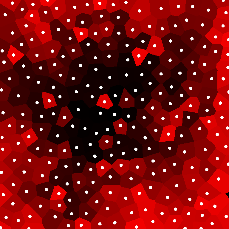
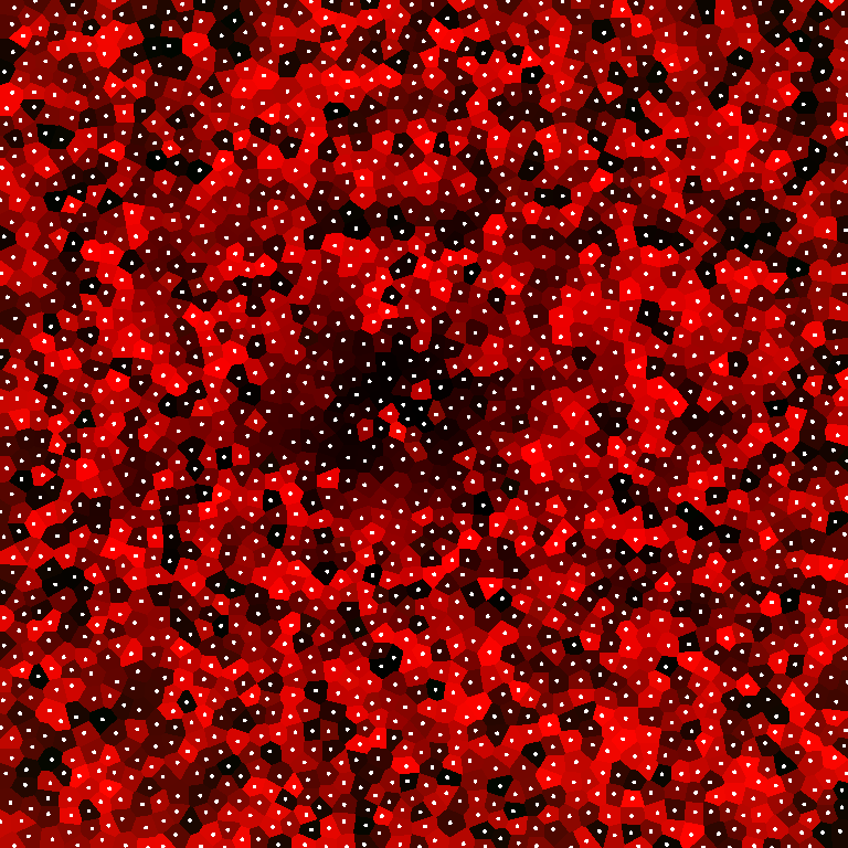
  if(style == 1) //Draw Depth
    fragColor = vec4(vec3(gl_FragDepth/R), 1.0);
  else           //Draw Labeling Map (Normal Voronoi Texture)
    fragColor = vec4(ex_Color, 1.0);

  if(gl_FragDepth < 0.1*R && drawcenter) //Draw Centroids
    fragColor = vec4(1.0);
}

That’s it! The rest of the code is just for adding centroids in the visualization or drawing the depth map instead.

Fragment Waste

Rendering a large amount of fragments only to discard them in the depth test is expensive, even if all fragments in an instance are given the same color. This ended up being the key performance factor.

The easiest way to fix this would be to make an assumption about the distribution of distances R between points. That way, the size of the quad can be reduced to side-length 2R.

A poisson disc generates points in a plane with a constraint on the distance between two points (“blue noise”). Such an assumption is justified for many applications, as it is more common for objects or particles to be spaced with uniform distance rather than uniformly in space.

Scaling the quad-size with the distance between samples means that the number of centroids can be scaled quite large without a significant performance penalty

I implemented a poisson disc sampler for generating a set of points in a region, and used this for generating the texture.

Note: My poisson disc sampler is not very good. Sometimes it fails, I don’t know why.

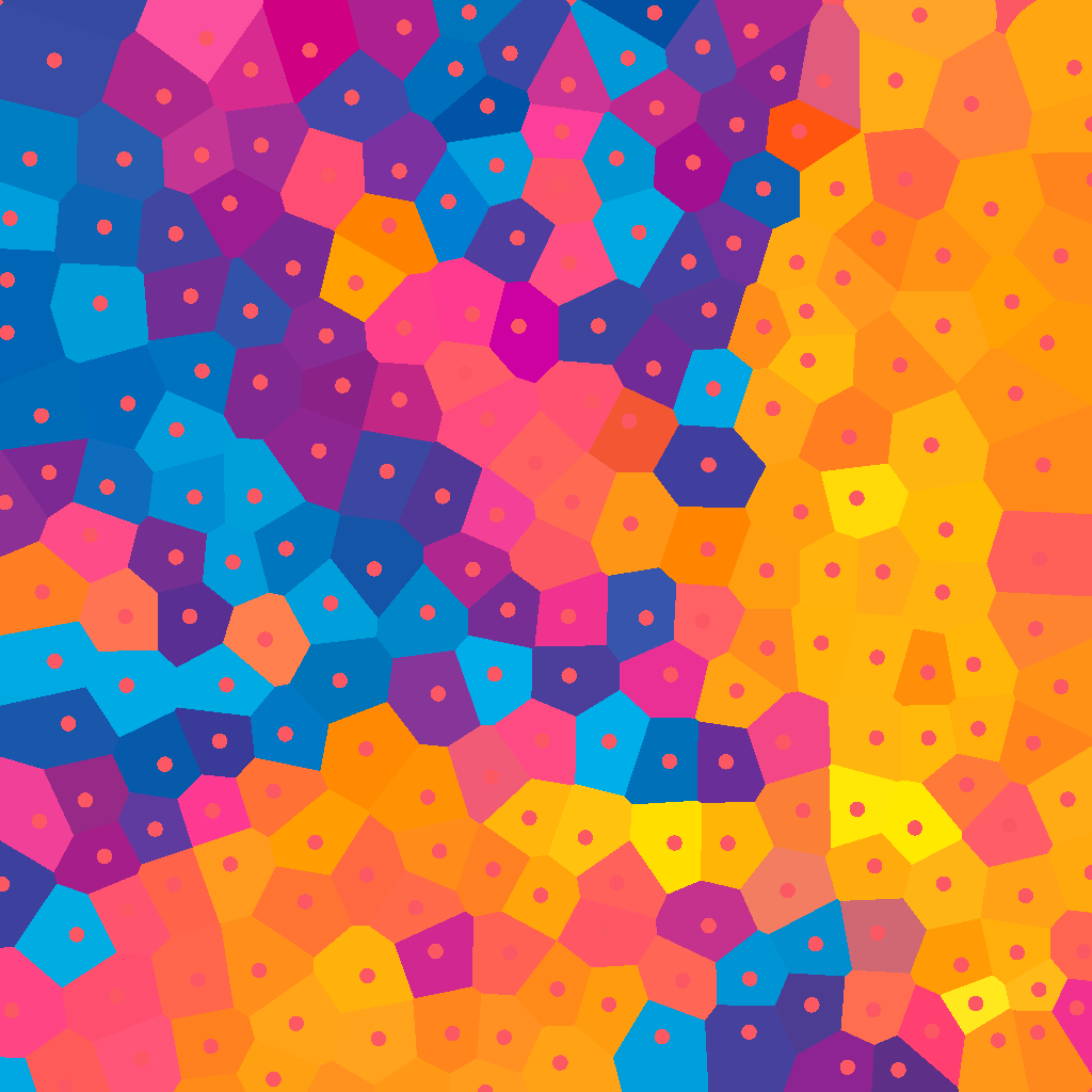
Results

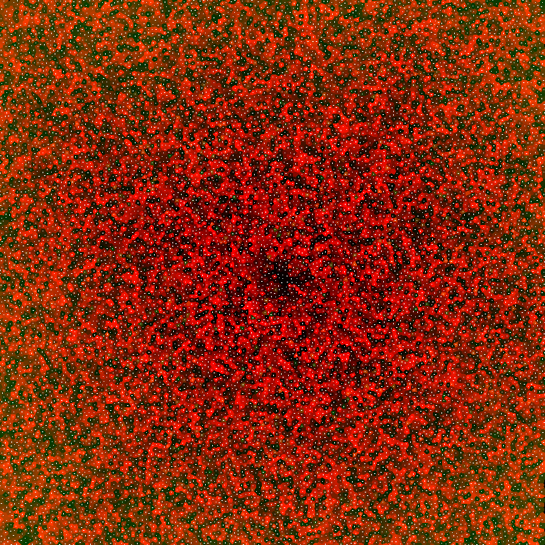
The shader generates a label image where each color corresponds uniquely to a centroid. The shader is very fast, so it is possible to update the centroid position every frame and redraw the entire diagram.

Recomputing the centroids using the poisson disc is relatively quick, so the number of centroids can also be changed at run-time, with no visible performance penalty.

There are some visual artifacts at the boundary because the poisson disc attempted to fill the space with too few centroids. This could be fixed with a better poisson disc sampler than mine (force in more points at boundary).

Performance

The shader performs very well at high resolutions and with high pixel counts. Here is a small amount of data that I generated on my Laptop running this program:

Node Number vs. Image Size	[512×512]	[768×768]	[1024×1024]
2^6	185 us	621 us	642 us
2^8	200 us	603 us	550 us
2^10	151 us	580 us	612 us
2^12	104 us	250 us	482 us
2^14	480 us	103 us	283 us
2^16	520 us	122 us	529 us

Note: I benchmarked specifically the part where I render using the voronoi shader. I applied glFlush() afterwards to guarantee an accurate timing. The values were consistent across different seedings of points. I have a laptop with an integrated GPU.

Interestingly, as the number of centroids rises, the program can actually become faster!

This tells me that the program does not care about the instancing, but cares very much about what is going on in the fragment shader, because we are drawing smaller quads.

Otherwise it is hard for me to detect any patterns, except that there clearly is some cache magic going on.

• 

• 

• 

Still: The shader is capable of generating a high resolution voronoi texture consistently in under a millisecond. This makes it very feasible for real-time applications and integration into other problems in the form of a shader. Nice.

Note: While this is very fast, it is not generalized because it assumes an average distance between points. This is the key limitation of this approach.

Comparison to other Algorithms

There are other methods for generating voronoi textures on the GPU, for instance using a grid-based approach (related to Worley-Noise).

This approach and related rely on an assumptions about centroid placement in a grid, while my method only requires an assumption about the maximum expected distance between two neighboring cells.

While my centroids are placed using a grid-based poisson disc, not every cell is guaranteed to contain a centroid.

Thereby, this approach is slightly more general in that it is agnostic about the structure of the centroids. This also eliminates all iteration in the fragment shader.

Because of this, this implementation will also NOT perform well for strongly clustering centroids (i.e. not evenly spaced, “white noise”), due to increased fragment waste. If centroids are spaced evenly (blue noise distribution – this assumption can be made in many applications), performance is better than other GPU based voronoi approaches (by 1-2 orders of magnitude!) that use jump flooding.

Other extensions to this algorithm, e.g. smoother distance metrics, are trivially implemented.

Voronoi Filters

The extreme performance means that it is possible to change the centroids and regenerate the voronoi texture every frame.

The color-labeling of the voronoi texture also allows us to compute the index of the centroid to which any pixel belongs. With this information, we can access the centroid position in the shader in constant time and use it for nice real-time visual effects!

This is realized by rendering to a separate FBO (with a depth and color buffer) in a voronoi pass, and using the texture to generate shader effects.

The index of the centroid any pixel belongs to can be accessed using the color sampled from the voronoi texture:

//... Filter Fragment Shader
#version 430 core
in vec2 ex_Tex;
out vec4 fragColor;

//Centroids Passed as SSBO
layout (std430, binding = 3) buffer centroids {
  vec2 c[];
};

int index(vec3 a){
  a = a*255.0f;
  return int((a.x + a.y*256 + a.z*256*256));
}

void main(){
  int i = index(texture(voronoi, ex_Tex).rgb);
  fragColor = filter_function_from_centroid(c[i]);
}

//...

Centroids are passed in a shader storage buffer objects.

For one, we can implement a dynamic mosaic effect by sampling an image at the centroid position (without offset):

If one imagines the voronoi regions as bubbles in a foam, individual bubbles can act as lenses to distort an image:

Other effects are certainly possible.

Final Words

The real-time capabilities of the voronoi shader are very nice, particularly with large numbers of centroids and relatively high resolutions. I don’t even have a real GPU.

Imagining the centroids as particles, it would perhaps be possible to generate nice visual effects in a flow-field or by giving them interacting properties.

This was a very quick proof of concept that I hope to explore further, particularly in relation to particle dynamics (voronoi / cluster-kernels in real time?) and physical system modeling.

This program is trivially extendable to e.g. a cube-map, for generating a voronoi texture on a sphere and doing related things.