Note: The full source for this project can be found [here]. Because this is part of a bigger project, I recommend looking at the commit at the time of this article’s release, or in “/source/helpers/arraymath.h”, as well as “/source/world/blueprint.cpp”.
In this article, I want to go into depth about the principles behind using Markov Chains and statistics to procedurally generate 3D buildings and other systems.
I will explain the (basic) mathematics behind how this works, and hope to make the explanation as general as possible so you can apply the concept elsewhere, for instance 2D dungeon generation. The explanation will be supported by images and source-code as much as possible.
This method is a general method for procedural generation of systems that fulfill certain requirements, so I encourage you to read at least to the bottom of the first section to consider if this might be useful for your application, as I explain what the requirements are below.
The results will be used in my voxel engine so task-bots can build buildings and then towns. Example at the very bottom!
The Foundation
Markov-Chains
Markov Chains are a sequence of states that a system moves through, described by transitions in time. The transitions between states are stochastic, and are thereby described by probabilities which are characteristic for the system.
Our system is described by a state space, which is the space of all possible configurations of our system. If our system is defined properly, we can also define transitions between the states as discrete steps.
Note that from one state of our system, there are often multiple possible discrete transitions, that will each lead to a different state of our system.
The probability of transition from state i to state j is:
![]()
The Markov Process is the process of exploring this state space, using the probabilities that we give it.
Important for Markov Processes is that they “have no memory”. This simply means that the probabilities of moving towards a new state from our current state is only dependent on the current state, and not any states that came before.
![]()
Example: Text Generation
Our system is a sequence of bits. Our state-space is all possible sequences of bits. A discrete transition would be flipping a single bit from 0 to 1 or 1 to 0. If our system has n bits, then from each state we have n possible transitions to a new state. The Markov Process would be the exploration of our state space by flipping the bits in our sequence using certain probabilities.
Example: Weather Prediction
Our system is the current weather. Our state-space is all possible states that the weather can be in (i.e. sunny, cloudy, rainy, etc.). A transition would be the switching from any state to another state, where we can define a probability of the transition (e.g. “what is the probability that given that today is sunny, tomorrow it will be rainy, regardless of what the weather was yesterday?”).
Markov-Chain Monte-Carlo Algorithms
Because the transitions between our states are governed by probabilities, it is also possible to define the probability of being in any state at “steady-state” (or as time goes towards infinity, the average amount of time we spend in a specific state). This is the underlying distribution of our states.
A Markov-Chain Monte-Carlo (MCMC) algorithm is then a method for sampling from our state-space. Sampling means selecting a state using its probability of selection, given the underlying distribution.
We say that the probability of being in a state is proportional* to some cost-function, which you can imagine gives a “score” to the current state our system is in. We say if the cost is low, then the probability of being in that state is high, and this relationship is monotonic. The cost function is given by:
![]()
Note: I am not sure if “proportional” is the correct word here, as we don’t necessarily have a linear relationship.
Sampling from the distribution of states will then return a configuration with a low cost (or a good score) with higher probability!
Even for an extremely large state-space (possibly infinite, but “countably infinite”), the MCMC algorithm will find a low-cost solution for us, no matter the complexity of the system as long as we give it enough time to converge.
Doing a state-space exploration like this is a common technique for stochastic optimization, and has many applications in fields like machine learning.
The Gibbs-Distribution
Note: If this section is non-intelligible for you, feel free to skip ahead. The implementation part will still be usable.
Once we have defined a cost for a possible state, how do we say what the probability of that state is?
Solution: The Gibbs Distribution is the maximum entropy distribution under a given set of constraints.
This essentially means that if we define a set of constraints on the probabilities of our system, then the Gibbs distribution makes the “least amount of assumptions” on the shape of our distribution.
Note: The Gibbs distribution is also the distribution with the least sensitivity towards variation in the constraints (under the metric of the Kullback-Leibler divergence).
The only constraint we place on our distribution of states is the cost function, so we use that in the Gibbs distribution to compute the probability of transitioning between states:
![Rendered by QuickLaTeX.com \begin{equation*} \[ P_{ij} = \exp(-\frac{R(j)-R(i)}{T})*\frac{1}{Z_i} \] \end{equation*}](https://nickmcd.me/wp-content/ql-cache/quicklatex.com-017700c97e8afc8e2fdd13dc9a195abb_l3.png)
Where Z is the partition function of the set of transitions from state i. This is a normalization factor to ensure that the probabilities of transitions from any state sum to 1.
![Rendered by QuickLaTeX.com \begin{equation*} \[ Z_i = \sum_j(P_{ij}) \] \end{equation*}](https://nickmcd.me/wp-content/ql-cache/quicklatex.com-0522308b986af07f233eb45aa3ae04f0_l3.png)
Note that if we decide that our next state is going to be the same state, the relative cost is zero, meaning the probability after normalization is non-zero (due to the form of the distribution with the exponential)! This means we need to include the possibility of not changing states in our set of transitions.
Note also that the Gibbs distribution is parameterized by a “computational temperature” T.
One of the key advantages of using probabilities to explore the state space is that it is possible for the system to transition to states that are actually more expensive (because they have non-zero probability of transitioning), making it a non-greedy optimization method.
Note that as the temperature approaches infinity, the probability of any single transition approaches one, such that when the set of probabilities of all transitions from a state are normalized, they become equally probable (or the Gibbs distribution approaches the uniform distribution), regardless of whether they cost more!
As the computational temperature approaches zero, then the transitions with a lower cost become much more probable, such that favorable transitions become more likely.
While we perform the state space exploration / optimization, we gradually lower the temperature. This process is called “annealing“. This way at the beginning, we can move out of local minima easily, and at the end, we pick better solutions.
When the temperature is sufficiently low, then all probabilities will approach zero, except for the no-transition probability!
This is because only the no-transition has a cost difference of zero, meaning there is actually no temperature dependency. Because of the form of the exponential, when T becomes 0 this will be the only probability with a non-zero value, such that after normalization, it becomes one. Our system will thereby converge to a stable point, meaning further cooling is no longer necessary. This is an intrinsic property of generating the probabilities using the Gibbs distribution.
The way our system converges can be tuned by changing the rate of cooling!
If you cool slower, then you will end up with a generally lower-cost solution (up to a degree), at the cost of more convergence steps. If you cool faster, then there is a higher probability your system will be trapped in a higher cost sub-region of the state-space early on, meaning you will get “less optimal” results.
The Markov process thereby doesn’t just generate random results, but tries to generate “good” results, and will generate “good” results with high probability!
Under the definition of arbitrary cost-functions, there doesn’t need to exist a unique optimum. This probabilistic optimization method will only generate an approximation for the optimum by attempting to lower the cost function, and due to the sampling, will generate different results every time (as long as the RNG is seeded differently).
The sampling process itself can be done using the inverse transform method on the probability mass function of our discrete set of transitions. I show how to do this later.
Procedural Generation
Why is this useful for procedural generation?
For certain systems, it can often be difficult to define a simple algorithm that generates good results, particularly for complex systems.
Defining arbitrary generation rules can not only be complex, but is restricted by our imagination and the handling of edge cases.
If our system fulfills a certain set of requirements, then applying MCMC allows us to not have to worry about coming up with an algorithm or rules. Instead we specify a method to generate any possible result, and choose a good one intelligently based on a score.
The requirements are:
- Our system can be in a discrete (possibly infinite) configuration of states.
- We can define discrete transitions between states.
- We can define a cost-function that scores the current state of the system.
Further down I will give some other examples that I have thought of where this might be applied.
Implementation
Pseudo-Code
In our implementation, we wish to do the following:
- Define the state of our system.
- Define all possible transitions to the next state.
- Compute the cost of our current state.
- Compute the cost of all possible (or a subset of) next states.
- Compute the transition probability using Gibbs distribution.
- Sample the transitions using the probabilities.
- Perform the sampled transition.
- Lower the computational temperature.
- Repeat until satisfied.
In pseudo-code, this MCMC algorithm looks like:
//MCMC Algorithm to Sample a State

T = 200; //Some computational temperature initial value
State s = initialState();
Transitions t[n] = {...} //n possible transitions
thresh = 0.01; //Convergence Criterion (on temperature)

//Iterate until the convergence criterion
while(T > thresh){

  //Compute the Current Cost of our State
  curcost = costfunc(s);
  newcost[n] = {0};     //Initialize newcost to 0
  probability[n] = {0}; //Initialize transition probability to 0

  //Compute the Probabilities
  for(i = 0; i < n; i++){
    newcost[i] = costfunc(doTransition(s, t[i]));
    probability[i] = exp(-(newcost[i] - curcost)/T);
  }

  //Normalize the Probabilities
  probability /= sum(probability);

  //Sample the Transition
  sampled = sample_transition(t, probability);

  //Do the transition
  s = doTransition(s, sampled);

  //Lower the Temperature
  T *= 0.975;
}
Generating 3D Buildings
State Space and Transitions
To generate buildings in 3D, I generate a number of rooms, with a volume described by a bounding box.
struct Volume{
  //Bounding Box Corners
  glm::vec3 a;
  glm::vec3 b;

  void translate(glm::vec3 shift);
  int getVol();
};

//Get the Total Volume
int Volume::getVol(){
  return abs((b.x-a.x)*(b.y-a.y)*(b.z-a.z));
}

//Move the Corners of the Bounding Box
void Volume::translate(glm::vec3 shift){
  a += shift;
  b += shift;
}
If I generate n rooms, then the state of my system is the configuration of the bounding boxes in 3D space.
Note that the possible configurations for these volumes are infinite, but countably so (they can be enumerated in infinite time)!
//Vector of Rooms (My system state!)
std::vector<Volume> rooms;

//Create N Volumes
for(int i = 0; i < n; i++){
  //New Volume
  Volume x;
  x.a = glm::vec3(0);
  x.b = glm::vec3(rand()%4+5); //Random Bounding Box

  //Add the the available rooms.
  rooms.push_back(x);
}

//...
The set of possible transitions would then be a shift of a room along one of the 6 directions in space by a single step, AND the “non-transition”:
//...

//Possible set of transformations
  std::array<glm::vec3, 7> moves = {
    glm::vec3( 0, 0, 0),  //No move also a possibility!
    glm::vec3( 1, 0, 0),
    glm::vec3(-1, 0, 0),
    glm::vec3( 0, 1, 0),
    glm::vec3( 0,-1, 0),
    glm::vec3( 0, 0, 1),
    glm::vec3( 0, 0,-1),
  };

//...
Note: Important is that you include the possibility for the system to remain in its current state!
Cost Function
I wanted the volumes in 3D space to act “magnetically”, meaning:
- If their volumes overlap, that’s bad.
- If their surfaces touch, that’s good.
- If they don’t touch at all, that’s bad.
- If they’re touching the floor, that’s good.
For two cuboid volumes in 3D space, it is possible to easily determine the bounding box:
Volume boundingBox(Volume v1, Volume v2){
  //New Bounding Volume
  Volume bb;

  //Determine the Lower Corner
  bb.a.x = (v1.a.x < v2.a.x)?v1.a.x:v2.a.x;
  bb.a.y = (v1.a.y < v2.a.y)?v1.a.y:v2.a.y;
  bb.a.z = (v1.a.z < v2.a.z)?v1.a.z:v2.a.z;

  //Determine the Upper Corner
  bb.b.x = (v1.b.x > v2.b.x)?v1.b.x:v2.b.x;
  bb.b.y = (v1.b.y > v2.b.y)?v1.b.y:v2.b.y;
  bb.b.z = (v1.b.z > v2.b.z)?v1.b.z:v2.b.z;

  return bb;
}
Using the bounding box of the volumes, I can compute a single 3D vector that gives me the overlap information of the two volumes.
If the length of the bounding box across one side is larger than the combined length of the two volumes across that side, then they don’t touch on that side. If it is equal, their surfaces touch exactly, and if it is smaller, then the volumes intersect.
//Compute the Volume Overlap in 3 Directions
glm::vec3 overlapVolumes(Volume v1, Volume v2){
  //Compute Bounding Box for the two volumes
  Volume bb = boundingBox(v1, v2);

  //Compute the Overlap
  glm::vec3 ext1 = glm::abs(v1.b - v1.a);  //Extent of v1 in 3 directions
  glm::vec3 ext2 = glm::abs(v2.b - v2.a);  //Extent of v2 in 3 directions
  glm::vec3 extbb = glm::abs(bb.b - bb.a); //Extent of the bounding box

  //Overlap is given
  return ext1 + ext2 - extbb;
}
This is used to compute a number of quantities over which I form a weighted sum, which finally acts as my cost.
int volumeCostFunction(std::vector<Volume> rooms){
  //Metric
  int metric[6] = {
    0, //Positive Intersection Volume
    0, //Negative Intersection Volume
    0, //Surface Area Touching Vertically
    0, //Surface Area Touching Horizontally
    0, //Amount of Area Touching Floor
    0};//Amount of Volume Below the Floor

  int weight[6] = {2, 4, -5, -5, -5, 5};

  //Compute the Energy of a configuration of rooms
  for(unsigned int i = 0; i < rooms.size(); i++){

    //Comparison Metrics to Other Rooms
    for(unsigned int j = 0; j < rooms.size(); j++){
      //If it's the same room, ignore.
      if(i == j) continue;

      //Compute the Overlap between two volumes.
      glm::vec3 overlap = overlapVolumes(rooms[i], rooms[j]);

      //Positive Intersection Volume
      glm::vec3 posOverlap = glm::clamp(overlap, glm::vec3(0), overlap);
      metric[0] += glm::abs(posOverlap.x*posOverlap.y*posOverlap.z); //Ignore Negative Values

      //Negative Intersection Volume
      glm::vec3 negOverlap = glm::clamp(overlap, overlap, glm::vec3(0));
      metric[1] += glm::abs(negOverlap.x*negOverlap.y*negOverlap.z); //Ignore Negative Values

      //Top Surface Contact
      if(overlap.y == 0){
        metric[2] += overlap.x*overlap.z;
      }
      //Side Surface Contact (X)
      if(overlap.x == 0){
        //This can still be 0, if it is corners touching, i.e. overlap.z = 0
        metric[3] += overlap.z*overlap.y;
      }
      //Side Surface Contact (Z)
      if(overlap.z == 0){
        //This can still be 0, if it is corners touching, i.e. overlap.x = 0
        metric[4] += overlap.x*overlap.y;
      }
    }

    //We need to know if any rooms are touching the floor.
    if(rooms[i].a.y == 0){
      //If the rooms is larger, than it is more important that it touches the floor.
      metric[4] += rooms[i].a.x*rooms[i].a.z;
    }

    //Check if we have volume below the floor!
    if(rooms[i].a.y < 0){
      //Check if the whole volume is below the surface
      if(rooms[i].b.y < 0){
        metric[5] += rooms[i].getVol();
      }
      else{
        metric[5] += abs(rooms[i].a.y)*(rooms[i].b.z-rooms[i].a.z)*(rooms[i].b.x-rooms[i].a.x);
      }
    }
  }

  //Return Metric * Weights
  return metric[0]*weight[0] + metric[1]*weight[1] + metric[2]*weight[2] + metric[3]*weight[3] + metric[4]*weight[4] + metric[5]*weight[5];
}
Note: “Positive Volume Intersection” means the volumes actually intersect. “Negative Volume Intersection” means they don’t touch at all, and is given by the volume of the space that is spanned by the two nearest points of the two cuboids in 3D space.
The weights are chosen in such a way that we promote certain things, and penalize other things. For instance, here I strongly penalize rooms that are below the floor, also strongly promoting surface area touching (more than I penalize volume intersections).
I form the cost for all pairs of rooms, ignoring rooms pairing with themselves.
Finding a low-cost solution
The convergence is done as described above in the pseudo-code. When I do a transition, I only move one room at a time. This means for n-rooms and 7 possible transitions, I have 7*n probabilities to compute, and I sample from all of these, only moving the room that is probably most favorable.
  //Computational Temperature
  float T = 250;

  while(T > 0.1){
    //Probability of Transition Array
    std::vector<std::array<double, moves.size()>> probabilities;

    //Compute the Current Energy (Cost)
    int curEnergy = volumeCostFunction(rooms);

    //Perform all possible transformations and compute the energy...
    for(int i = 0; i < n; i++){
      //Create the Storage Array
      std::array<double, moves.size()> probability;

      //Loop over the possible moveset, compute the probability of that transformation
      for(unsigned int m = 0; m < moves.size(); m++){
        //Translate the Room by the move and compute the energy of the new configuration.
        rooms[i].translate(moves[m]);

        //Compute the transition probability using the energy difference!
        probability[m] = exp(-(double)(volumeCostFunction(rooms) - curEnergy)/T);

        //Translate it Back
        rooms[i].translate(-moves[m]);
      }

      //Add the probabilities for this room to the vector
      probabilities.push_back(probability);
    }

    //Partition Function (Normalization Factor)
    double Z = 0;
    for(unsigned int i = 0; i < probabilities.size(); i++){
      for(unsigned int j = 0; j < probabilities[i].size(); j++){
        Z += probabilities[i][j];
      }
    }

    //Normalize the Probabilities
    for(unsigned int i = 0; i < probabilities.size(); i++){
      for(unsigned int j = 0; j < probabilities[i].size(); j++){
        probabilities[i][j] /= Z;
      }
    }

    //Compute the Cumulative Density Function (for sampling)
    std::vector<double> cdf;
    for(unsigned int i = 0; i < probabilities.size(); i++){
      for(unsigned int j = 0; j < probabilities[i].size(); j++){
        if(cdf.empty()) cdf.push_back(probabilities[i][j]);
        else cdf.push_back(probabilities[i][j] + cdf.back());
      }
    }

    //Generate uniform random variable
    std::random_device rd;
    std::mt19937 e2(rd());
    std::uniform_real_distribution<> dist(0, 1);
    double uniform = dist(e2);
    int sampled_index = 0;

    //Sample from the CDF
    for(unsigned int i = 0; i < cdf.size(); i++){
      //If we surpass the value of uniform, we have found the guy...
      if(cdf[i] > uniform){
        sampled_index = i;
        break;
      }
    }

    //Determine Sampled Room and Move
    int _roomindex = sampled_index/moves.size();
    int _moveindex = sampled_index%moves.size();

    //Perform the Move
    rooms[_roomindex].translate(moves[_moveindex]);

    //Lower T
    T *= 0.99;

    //Repeat!!!
  }
//Done!!

//...
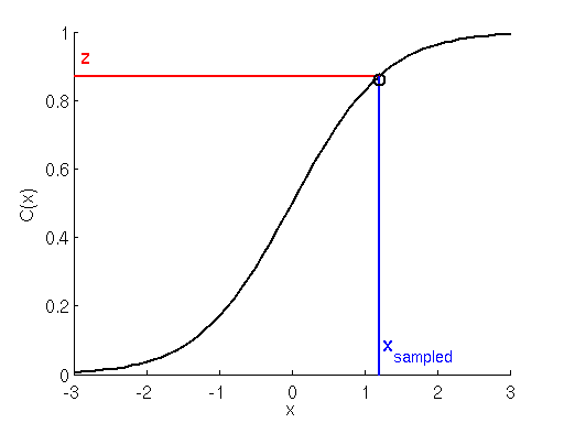
The sampling is done by forming the cumulative distribution function over the probability mass function of all possible transitions, and doing what is called “inverse transform sampling”.
This works by forming a cumulative sum over the probabilities of our transitions, giving us our “cumulative distribution function” (CDF). To sample, we generate a uniform random variable between 0 and 1. Because the first entry of the CDF is zero, and the last entry is 1, we simply need to find “at what index in the CDF array our uniformly sampled variable lies”, and that is the index of the sampled transition. Here is an illustration:
Finally, I have the volume data of my rooms in 3D space!
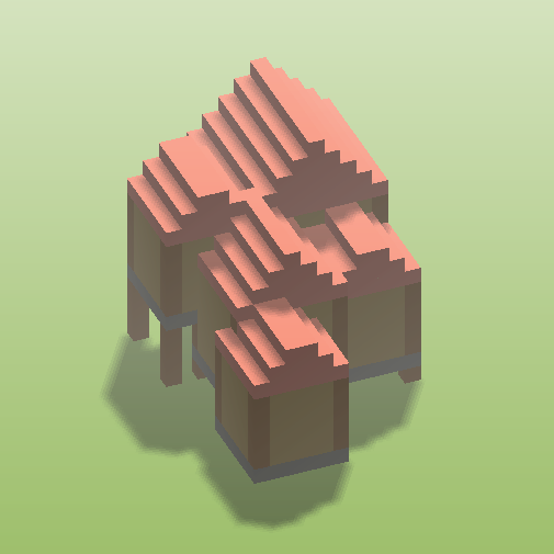
I use this to generate a blueprint using my blueprint class, applying a theme to the known volumetric data! This gives the houses their appearance. The blueprint class is described in a previous article [here]. See the source code for the full generation of the house from the volumes data.
Results
This gives pretty good results for a general method. The only real tuning I had to do was ensure that my cost-function was promoting and penalizing the right things with the correct weights.
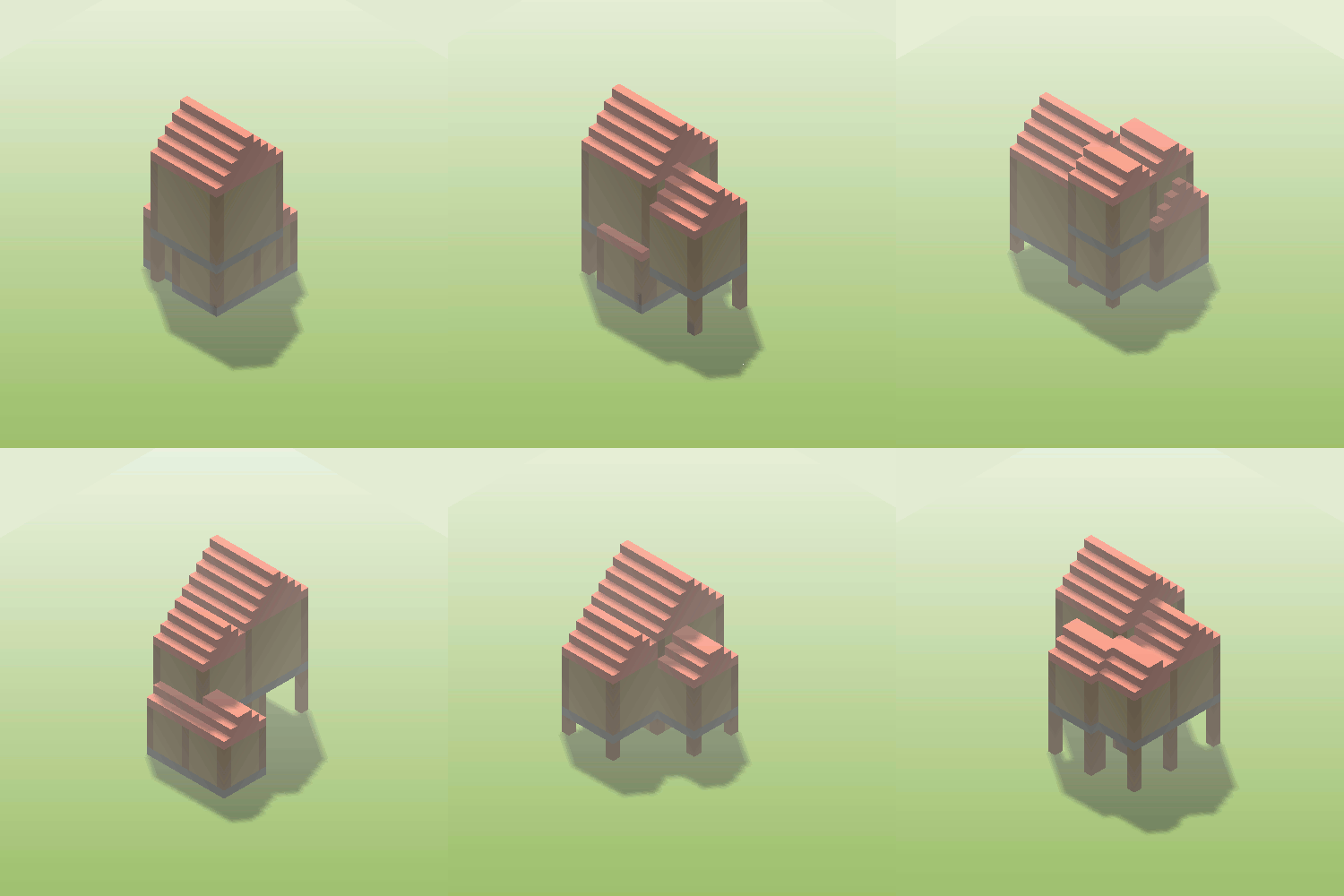
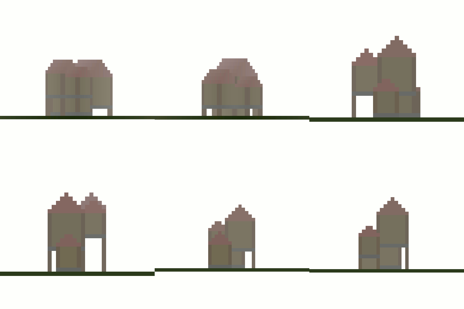
The convergence itself is very fast, particularly for small numbers of rooms (3-5), because the bounding box calculations and the cost function evaluation are very simple.
In the current state, houses don’t have doors and windows, but that is more a question of interpreting the 3D volume data and not something that affects the underlying MCMC algorithm.
The method can sometimes give wonky results, as it is a stochastic process, so it is important that some sanity checks are applied to the result before it is placed in the world, particularly if the cost function isn’t very robust. I suspect that the wonkyness mostly occurs in the first few steps of the iteration when the temperature is high.
Wonkyness typically includes detached rooms, and rooms floating high up in the air (on giant stilts).
Expansions and Other Systems
It is clear that my 3D volume method could easily be translated into a 2D method, by simply reducing the dimensionality of the problem by one.
It could thus be applied to things like procedural dungeon generation, or rooms in 2D top-down games, by attaching rooms to each other using a cost function similar to the one I defined.
A possible method to make the room generation more interesting would be to first generate a graph of rooms, each with different types, and then defining a cost-function which promotes the connectivity of rooms that are connected in the graph via physical surfaces.
The graph itself could be generated using an MCMC algorithm, with the making and breaking of connections between rooms considered the discrete transitions, promoting connections between rooms of certain types (bedrooms more likely connected to hallways, less likely connected to the outside, etc).
Other possible applications include:
- Maze generation, defining cost over tortuosity in the maze, and transitions being the placement / removal of walls or hallways.
- Road networks, linking and destroying connections between nodes in a graph based on distance, terrain, or other factors as cost.
- Probably much more!
Fun side-note: Simulated annealing and MCMC algorithms can be applied to problems like “traveling salesman”, a famous NP hard problem. The state of the system is the path, transitions could be switching out nodes on the path, and the cost is the total distance!
Implications for Task-Bots
Using this, I hope that task-bots can draft their own buildings in the future according to their requirements.
Since the MCMC algorithm consists of discrete convergence steps, I picture one convergence step corresponding to a single “draft” task, so that a bot can perform the convergence slowly and take their time.
Here is a video of a bot building a house generated using this algorithm:
Final Words
I tried to make this understandable while not trying to rely on any “this is magic – trust me”. Still, if you have questions, or want a more in depth explanation on how this works, or how you could apply it to a specific system, then feel free to contact me.
I hope this can act as a resource to people trying to procedurally generate stuff, while using some robust statistical methods!
