Note: The source code for this project can be found [here].
One of the key goals of procedural terrain is the generation of a realistic heightmap representing the topography. In real systems, the topography has a strong coupling to a number of surface phenomena, e.g. hydraulic erosion, plant growth, wind erosion, etc. which yield the “topographical realism”.
A large variety of techniques exist to generate height-maps with one-way couplings to such surface phenomena: For instance generating a height-map by sampling continuous noise and identifying rivers using gradient descent, or generating rivers using a space-filling curve and extracting the required topography.
Particle-based erosion methods offer a good compromise by coupling topology and surface phenomena in both ways, without excessive complexity and strong potential for realism if implemented properly.
Most procedural methods for topography generation at some point rely on applying continuous noise functions, for instance as an “initial topography”. The sampling from such noise functions represents a strong assumption which is difficult to physically justify.
Note: A statistical argument is often made for noise sampling e.g. from fractal-brownian-motion in some circumstances, but this comes with its own limitations. The assumption is then that “the topography follows a distribution which can be sampled”. If such a distribution exists, it emerges due to the real dynamics.
In this article I would like to explore the idea of eliminating the noise sampling from the “initial topography” by asking: “Where does non-eroded rock come from in the first place?”
I will describe my (third) attempt at implementing a simple plate-tectonics simulation for generating the initial terrain for (later) utilization with an erosion-based system.
I utilize a technique I call “clustered convection“. The idea is to approximate the dynamics of a continuous field (i.e. the topography) using a dynamic / deformable point cloud, which become centroids in a clustering. This has a number of advantages in dealing with “rigid structures” like tectonic plates while offering a lot of additional flexibility.
The system can handle deformable and arbitrarily shaped plates with non-uniform properties in real-time.
I attempt to explain my implementation in detail with code samples in C++ and GLSL.
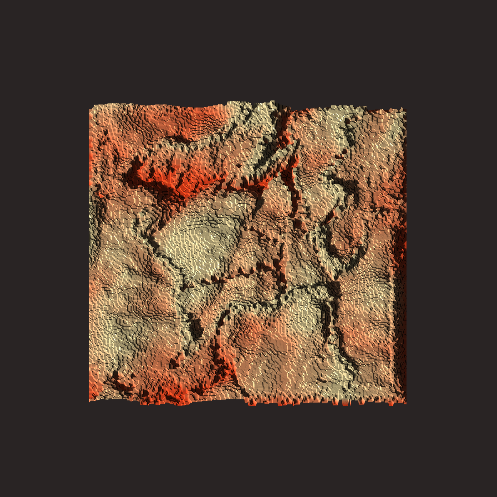
Plate Visualization 1 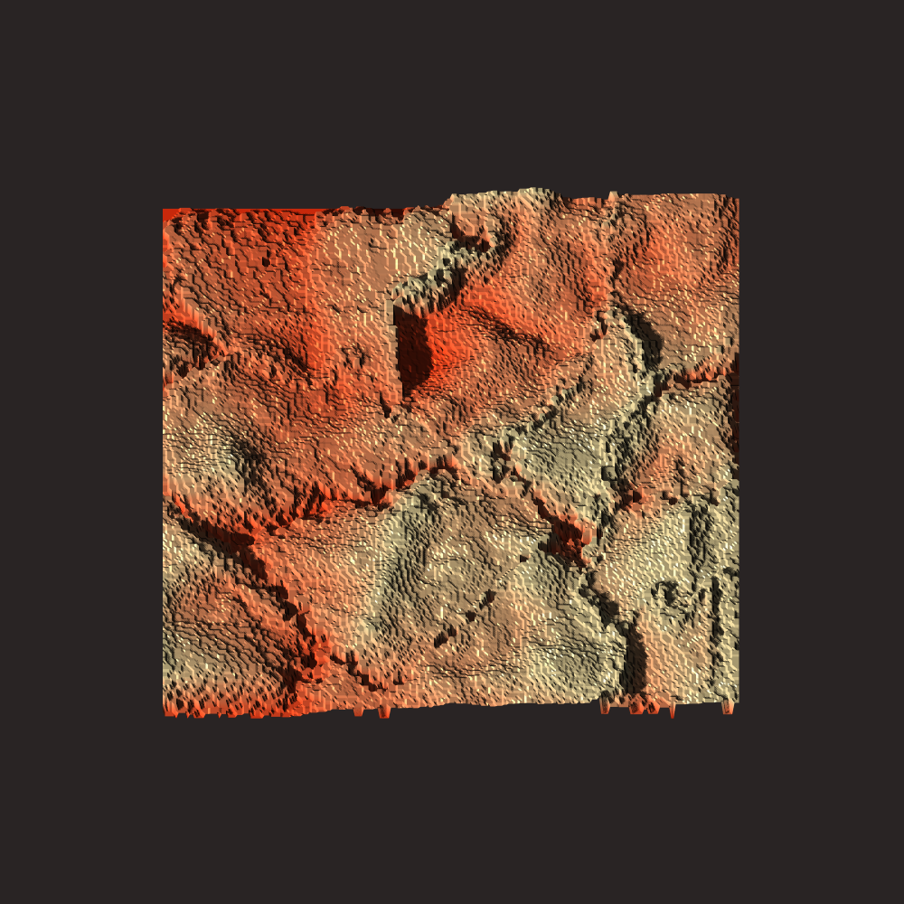
Plate Visualization 2 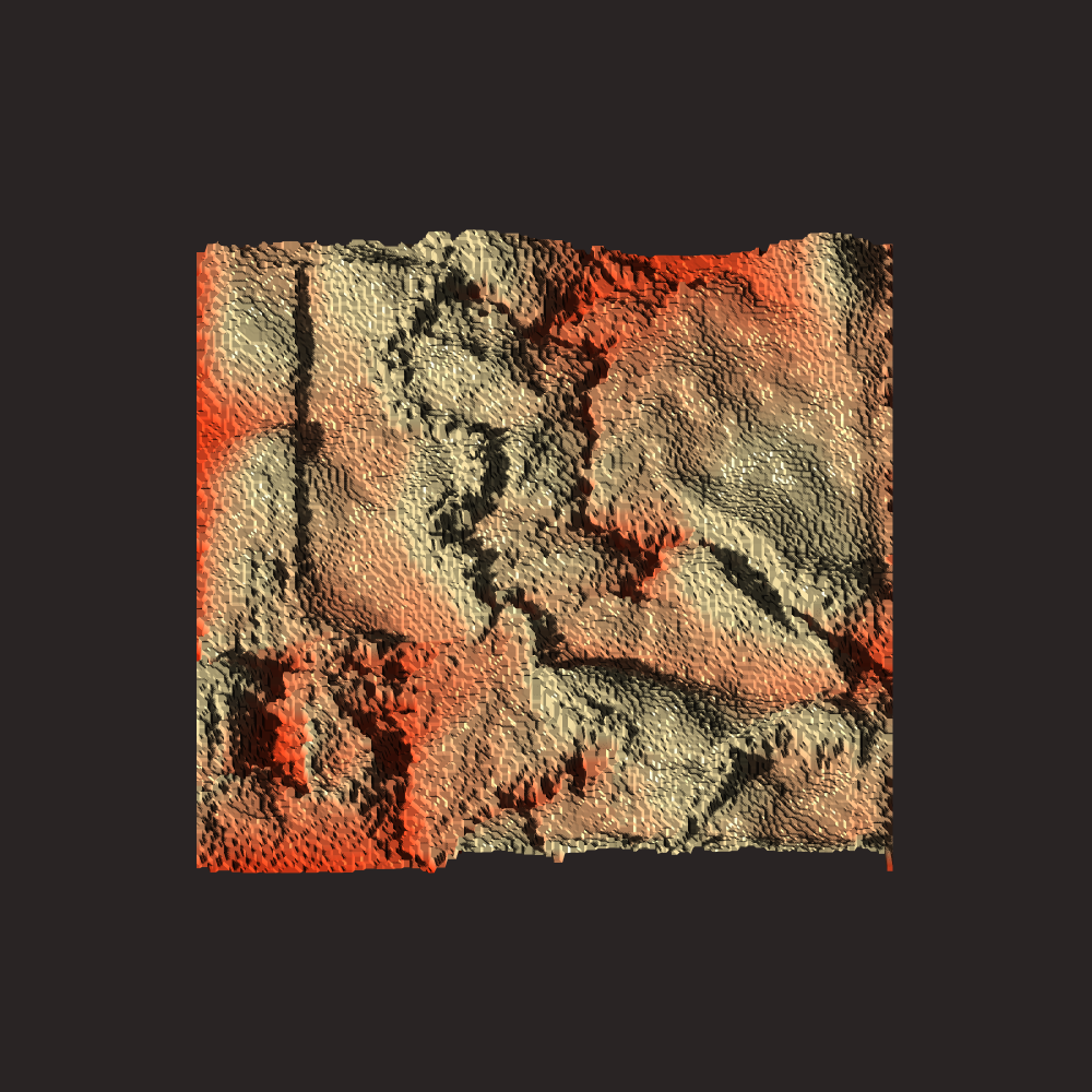
Plate Visualization 3 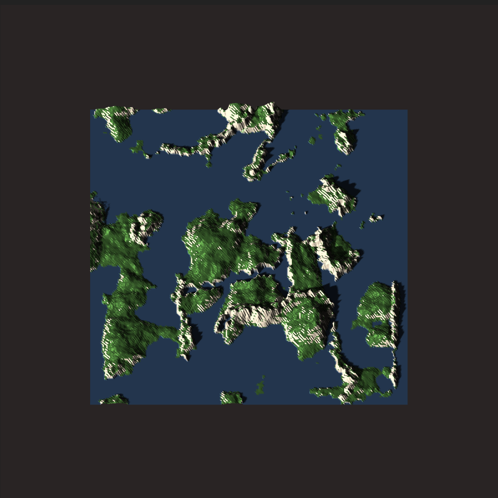
Terrain Visualization 1 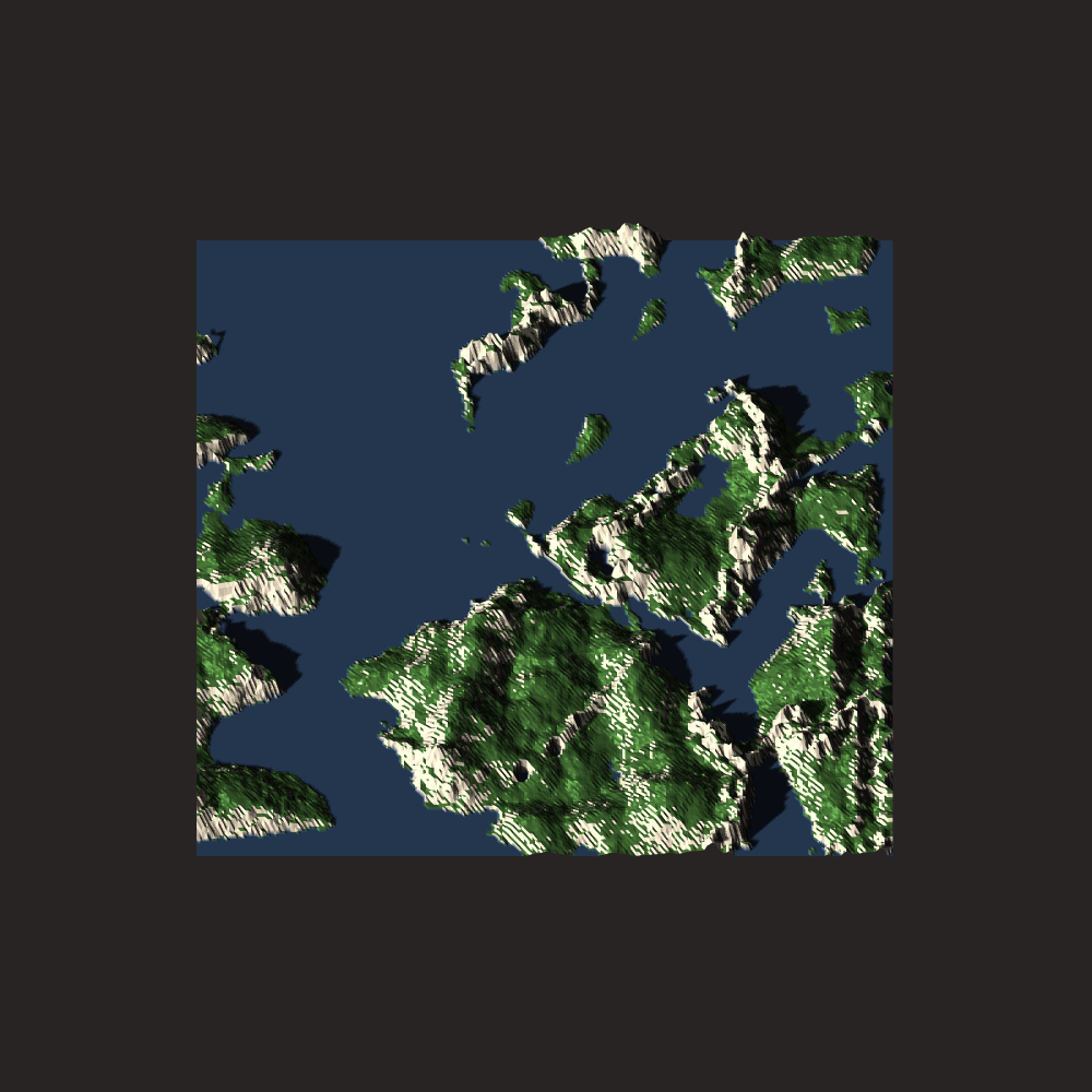
Terrain Visualization 2 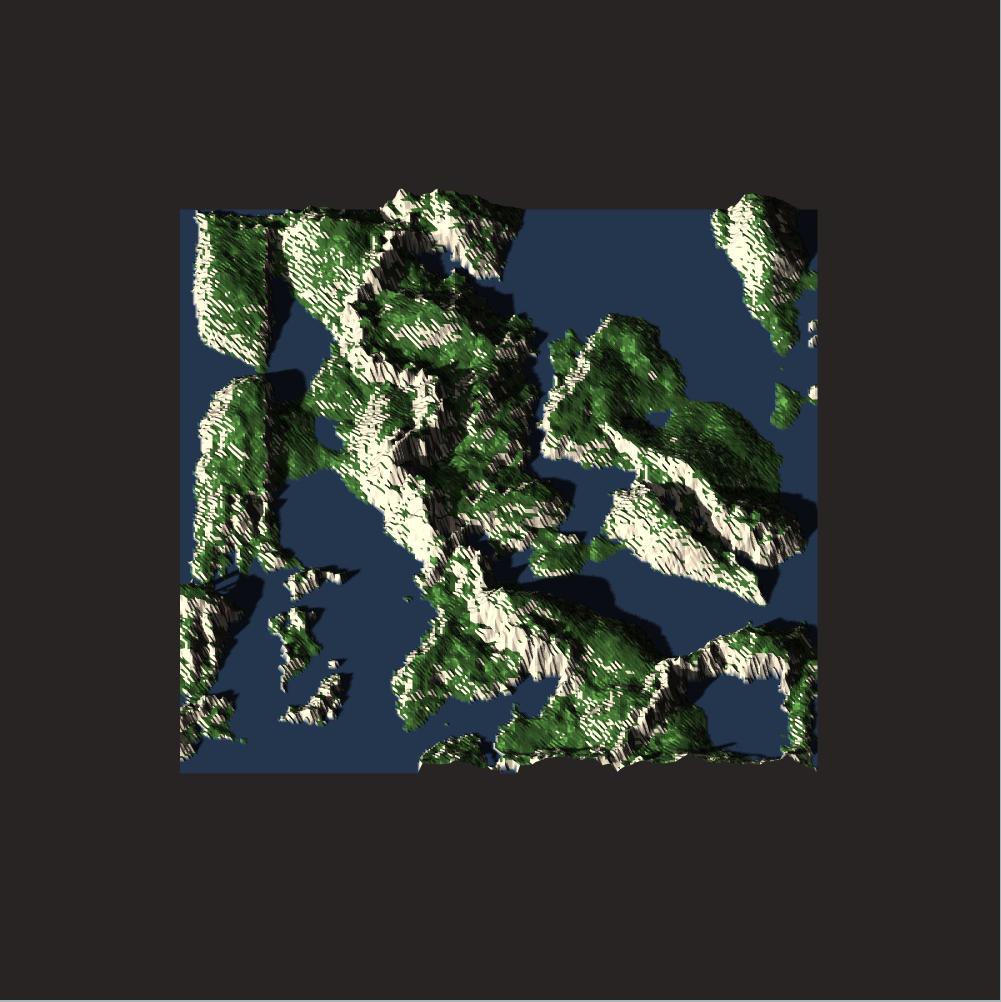
Terrain Visualization 3
Overall the code required for the clustered convection is about 130 lines of code and the code required for the actual plate tectonics is currently just under 600 lines of code (but I think I can cut this down dramatically in the future).
Note: Clustered convection is a technique I have been thinking about for a while but which has recently become possible to implement due to GPU accelerated voronoi shaders and filters. This system makes heavy use of GLSL shaders and GPU parallelization and is therefore “intermediate difficulty”. The technique is still implementable without OpenGL / GPU programming but it will be significantly slower.
Simulating Plate Tectonics
A number of existing projects simulate plate tectonics by simulating the movement of groups of points on a grid and finding intersections to place sediment using distributions.
Examples for Alternative Methods: https://tectonictiles.wordpress.com/?order=asc
Other approaches instead split the map into an irregular set of cells, for instance a voronoi tessellation, representing the plates. The fundamental idea behind such approaches is that the plate moves as a quasi-rigid body, with most dynamics happening at the boundary, so “labeling” using cells makes it easy to describe dynamics over a large, continuous area.
The main issue with this approach is that (without further assumptions) it models the plate with uniform properties across its entire area, for instance height, density, etc, with sharp and non-deformable boundaries.
Additionally, describing the motion of a rasterized label map is not trivial and requires many additional assumptions. For a voronoi labeling you can just move the centroid and re-label at every time-step, but this ruins all boundary dynamics.
I take a slightly different approach which is described below.
Clustered Convection
The description of plate motion can be simplified greatly by approximating every plate not as a clustering around a single point, but as a collection of evenly-spaced point clusterings.
The individual points are given dynamic properties which are considered representative in their “region of influence”, i.e. the area of their clustering. In this manner, any continuous field (e.g. a height-map) is approximated by a point cloud.
The convection on the continuous field is also simplified as points move around individually with their properties, while the clustering can be recomputed at every time-step without full loss of boundary dynamics.
The system has a few additional nice properties:
- Points can be added dynamically to regions with low density or removed from high density areas
- Individual points can have arbitrary movement
- Individual points can arbitrarily interact with others
- Individual points can easily interact with fields
Specifically for plate tectonics, this allows us to have plates of arbitrary shape which can be actively deformed and can still have properties which are not uniform across the plate.
Note: One nice implementation on a sphere uses an approach very similar to mine!
Implementation
Note: The source code specifically for clustered convection system can be found [here]. I use my homemade TinyEngine to interface with OpenGL, but the concept is portable to any GL.
To implement clustered convection, we need a few things:
- A storage system for points and their properties
- A method for generating a label map over our field
- A system for giving points dynamic properties
The label map is generated using a GPU Accelerated Voronoi shader. This process is relatively simple: We execute an instanced render over the set of 2D points and use the z-buffer to perform conic intersections. The color corresponds to an index by using the bits of the RGB color:
// GLSL VORONOI VERTEX SHADER
#version 430 core

//...

flat out vec3 ex_Color;
flat out int ex_InstanceID;

//Index to Color
vec3 color(int i){
  float r = ((i >>  0) & 0xff); //Shift by 0
  float g = ((i >>  8) & 0xff); //Shift by 256
  float b = ((i >> 16) & 0xff); //Shift by 256*256
  return vec3(r,g,b)/255.0f;    //Normalize between [0,1]
}

//Color to Index
int index(vec3 c){
  c *= 255.0f;
  return int((int(c.x) << 0) + (int(c.y) << 8) + (int(c.z) << 16));
}

//...

void main(){
  //...
  ex_Color = color(gl_InstanceID);
  ex_InstanceID = gl_InstanceID;
  //...
}
Note: This process has been described in detail in another blog article of mine so I won’t elaborate much more.
This produces a detailed label map where every cell in a grid with the size / resolution of the texture has a centroid. We can thus easily sample the index of the centroid each point belongs to using the inverse index formula.
Every point in the clustering has two default properties: A centroid position and an area. We combine these two key properties in a struct called a “Segment”.
struct Segment {
  Segment(vec2* p):pos{p}{}
  vec2* pos = NULL;           //Segment Position
  int area = 1.0;             //Area of Segment (Pixels)
};
Note: The area is initialized to 1 because each centroid belongs to at least 1 pixel. Also no division by zero.
To specialize the segments for a specific purpose, we can then define a derived class with additional members.
We store the point set, segments, label map and the OpenGL code required to generate it in a class “Cluster”. Note that this is templated by the segment’s derived class.
We define some convenience functions for adding a segment at a specific position, removing all segments satisfying a condition and sampling the label map:
#define SIZE 256

template<typename T>
class Cluster {
public:

vector<vec2> points;     //Raw Centroid Data
vector<T*> segs;         //Raw Segment Structs
int* indexmap;           //Flattened 2D Index Array

T* add(vec2& p);         //Add a Segment from a Point
void remove(function<bool(T*)> f); //Remove on Condition
int sample(vec2 p);      //Sample Indexmap at 2D Position

//...
For the clustering system to work, the points should be in contiguous memory. Therefore the clustering stores a vector of points and segments store a pointer to that point. A reassign function makes sure the references are correct, as they can change due to vector reallocation.
Note: The pointer invalidation / reassignment is actually one of this system’s main flaws. I have a concept for how this issue can be eliminated entirely but it requires a rewrite of my TinyEngine code which I am too lazy to do right now. I will probably tackle this in the future though. I discuss this at the end of this article.
In the Cluster constructor, we set up the clustering system, sample the points in our domain and add the segments.
Note: To understand the components of the clustering system you can read GPU Accelerated Voronoise.
//...

void reassign();         //Reassign Segment References
void update();           //Recompute Clustering

Square2D* flat;          //2D Billboard
Instance* instance;      //Instanced Rendering Helper
Billboard* target;       //FBO for Rendering Label Map
Shader* voronoi;         //Clustering Shder

Cluster(){

  indexmap = new int[SIZE*SIZE];

  flat = new Square2D();
  instance = new Instance(&*flat);     //Instance Wrap Flat
  target = new Billboard(SIZE, SIZE);  //Size of Domain

  voronoi = new Shader( {"voronoi.vs", "voronoi.fs"}, {"in_Quad", "in_Tex", "in_Centroid"}, {"area"}); //2 Shader Files, 2 Model Properties, 1 Instanced Property, 1 SSBO

  //Poisson Disc Sample in our Domain
  sample::disc(points, K, vec2(0), vec2(SIZE));
  for(auto&c : points) add(c); //Add Points

  instance->addBuffer(points); //Add the Instanced Buffer
  update();

}

~Cluster(){

  delete target;
  delete[] indexmap;
  delete voronoi;
  delete instance;
  delete flat;

  for(int i = 0; i < segs.size(); i++)
    delete segs[i];

}

};
Note: The points are generated using my poisson disc sampler.
The update function then generates and stores the label-map based on our point set:
template<typename T>
void Cluster<T>::update(){

  vector<int> area;              //SSBO for Area Accumulation
  for(size_t i = 0; i < segs.size(); i++)
    area.push_back(0);           //Initialize to Zero
  voronoi->buffer("area", area); //Add the SSBO

  //Update Instance with Point-Set
  instance->updateBuffer(points, 0);

  //Render Voronoi Texture
  target->target(vec3(1));
  voronoi->use();
  voronoi->uniform("R", R);             //Centroid Radius
  voronoi->uniform("depthmap", false);
  instance->render();

  //Extract the Index Map
  target->sample<int>(indexmap, vec2(0), vec2(SIZE, SIZE),
                      GL_COLOR_ATTACHMENT0, GL_RGBA);

  //...
Note that the voronoi shader takes the centroids as an instanced buffer, but also receives an SSBO which contains the areas of the segments. The reason for passing this as an SSBO is so that the voronoi fragment shader can perform an atomic add operation for every pixel belonging to a given centroid, leading to a fast parallel area computation:
//GLSL VORONOI FRAGMENT SHADER
#version 430 core

flat in int ex_InstanceID;
//...

layout (std430, binding = 0) buffer area {
  int a[];
};

void main(){

  //Assign color...

  atomicAdd(a[ex_InstanceID], 1); //Accumulate Area

}
The areas are then extracted by mapping the SSBO:
//...

  //Extract per-segment Area
  glBindBuffer(GL_SHADER_STORAGE_BUFFER, voronoi->ssbo["area"]);
  int* areapointer = (int*)glMapBuffer(GL_SHADER_STORAGE_BUFFER, GL_READ_ONLY);
  for(size_t i = 0; i < segs.size(); i++) //Rolling Update (Less Noise)
    segs[i]->area = segs[i]->area*0.99 + 0.01*areapointer[i];
  glUnmapBuffer(GL_SHADER_STORAGE_BUFFER);

} //End of Update function
Note: I use a rolling update scheme on the area value because the clustering can lead to noisiness otherwise.
In principle, this is all that is needed for clustered convection. Each segment is now associated with a point and an area, and a full index map has been computed. This process is also extremely fast due to full GPU parallelization.
To utilize such a system most generally, the points need to be given a description of motion and how their properties interact with any continuous field they exist in.
Note: Some additional optimizations would be possible by applying persistently mapped buffers and vertex pooling.
Plate Tectonics Model
Note: The code for this part of the article can be found [here].
At the core of plate tectonics lies a crystallization process on the surface of the earth’s asthenosphere (a deformable sub-layer), forming the lithosphere, the more rigid surface layer of hard rock. This layer undergoes fracturing and the individual “plates” then convect on the surface, while interacting at boundaries and with the asthenosphere below.
The thickness of the lithosphere is dependent on the temperature of the asthenosphere below. Cold regions of the asthenosphere lead to crystallization of rock at the bottom surface of the lithosphere, and warmth conversely leads to dissolution. The lithosphere then grows at the bottom with a varying density, depositing more dense rock when it is colder and less dense rock when it is warmer.
The asthenosphere is more elastic and undergoes a form of viscous flow. We can imagine that the lithosphere fractures (plates) “float” on the asthenosphere. The motion of plates is classically related to convective forces in the asthenosphere which result from differences in density (due to heat and mass), transferred to the plates via friction.
Note: Modern theory apparently states that gravity is also a major driving force, but I do not consider it in this model.
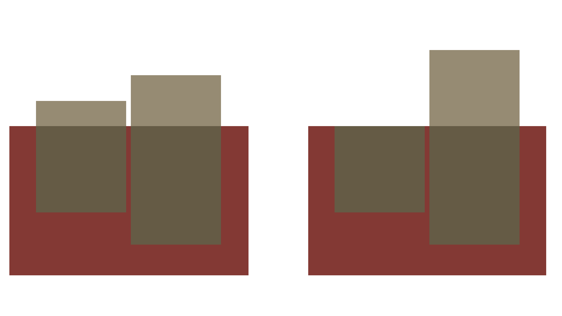
When two plates collide, the more dense / heavy plate will typically subduct under the less dense / lighter plate. This is phenomenologically observed as “ocean plates” subducing under “continental plates”, which are thicker and less dense.
When plates separate, new lithosphere will form at the opening via rapid cooling at the surface.
There are therefore three key things I wish to model:
- Growth of Plate Thickness by Cooling Crystallization
- Motion of Plates due to Convective Forces
- Convergent and Divergent Boundary Interactions
My descriptions and their implementations are shown below.
Model Outline
I simulate the world on a fixed-size grid with a height map and a heat map. The heat map summarizes the temperature and density properties of the asthenosphere, from which I can derive crystallization rates and densities, as well as convective forces. This is described in more detail later.
Note: To be more physically accurate, you can think of the heat map more as an “energetic potential” map or similar as it summarizes heat and density properties.
Segment Crystallization and Growth
Each segment undergoes a dynamic crystallization process while it floats independently on the asthenosphere.
We describe a lithosphere segment struct by giving it a total crystallized rock mass and a thickness. From this we can compute a density and a buoyant height at which it “floats” above the surface assuming an asthenosphere density of 1.
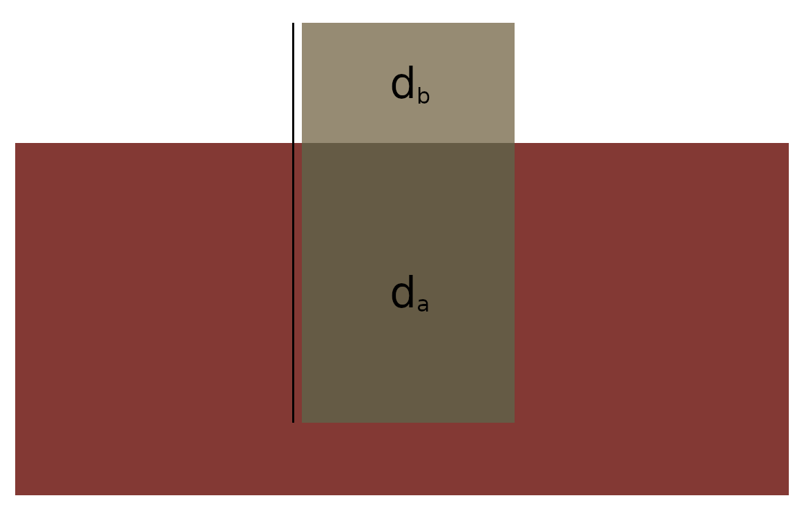
If a plate has thickness d, mass m and area A, (and density rho) the height floating above the surface is given by:
(1) 
while the height below the surface is given by:
(2) 
struct Litho : Segment {

  Litho(vec2* p):Segment(p){}    //Constructor

  vec2 speed = vec2(0);       //Velocity of Segment

  float mass = 0.1f;          //Absolute Accumulated Mass
  float thickness = 0.1f;     //Total Thickness of Plate

  float density = 1.0f;       //Density of Mass in Plate (Derived)
  float height = 0.0f;        //Protrusion Height (Buoyant) (Derived)

  //Compute Derived Quantities
  void buoyancy(){
    density = mass/(area*thickness);
    height = thickness*(1.0f-density);
  }

  bool alive = true;          //Segment Status
  bool colliding = false;

};
We describe the growth of a segment by defining an “equilibrium thickness” and an “equilibrium density” in dependency of the heat-map temperature T.
We say that at equilibrium the submerged segment thickness decreases linearly with the temperature. Additionally, we say that the growth rate decreases linearly with the temperature, implying faster growth / crystallization at lower temperatures. This gives us an overall growth rate expression G in m/s:
(3) 
To model the addition of mass, we define an equilibrium density D, which is the density at which the mass at the bottom of the lithosphere deposits. We say that at lower temperatures the deposit is more dense, approaching some maximum value. We can model this easily using a simple Langmuir isotherm:
(4) 
Note: There is no particular reason to use a Langmuir isotherm. You can use whatever you like.
We apply this equilibrium model to each segment and update its derived properties:
for(auto&s: seg){

  if(!s->alive) continue;

  ivec2 ip = *(s->pos);
  float temp = hm[ip.y+ip.x*SIZE]; //Heat Value!

  float rate = growth*(1.0-temp);
  float G = rate*(1.0-temp-s->density*s->thickness);
  if(G < 0.0) G *= 0.05;  //Dissolution Rate is Lower

  //Equilibrium Growth Density
  float D = langmuir(3.0f, 1.0-nd);

  //Grow Segment
  s->mass += s->area*G*D;
  s->thickness += G;

  //Recompute Density / Float Height
  s->buoyancy();

}
Note that the dissolution rate (i.e. G<0) is lowered by a factor. This produces the following motionless effect:
Note that this approach does not intrinsically differentiate between continental and oceanic plates but instead models the differences in plate density over time directly.
Segment and Plate Motion Description
In general, we describe the plates and their fracturing using groups of segments. A plate struct contains a vector of pointers to segments and has a number of properties describing its translation and rotation:
struct Plate {

  Plate(vec2 p):pos{p}{}

  vector<Litho*> seg;

  vec2 pos = vec2(0);    //Translation Properties
  vec2 speed = vec2(0);
  float mass = 0.0f;

  float rotation = 0.0f; //Rotation Properties
  float angveloc = 0.0f;
  float inertia = 0.0f;

  //Parameters
  float convection = 10.0f;
  float growth = 0.05f;

  void recenter(){

    pos = vec2(0);
    inertia = 0.0f;
    mass = 0.0f;

    for(auto&s: seg){
      pos     += *s->pos;
      mass    += s->mass;
      inertia += pow(length(pos-*(s->pos)),2)*(s->mass);
    }

    pos /= (float)seg.size();

  }

  void update(Cluster<Litho>&, double* heatmap);

};
A recenter function computes the plate’s center of mass, its total mass as well as its rotational moment of inertia. The update function then computes the motion of the plate.
We store a vector of plates with centers initialized at random positions. We then assign centroids to the nearest plate:
//...

//Generate Plates
vector<Plate> plates;

for(int i = 0; i < nplates; i++)
  plates.emplace_back(Plate(vec2(rand()%SIZE,rand()%SIZE)));

//Assign Segments to Plates
for(auto s: cluster.segs){

  float dist = SIZE*SIZE;
  Plate* nearest;

  for(auto&p: plates){
    if( glm::length(p.pos-*(s->pos)) < dist ){
      dist = glm::length(p.pos-*(s->pos));
      nearest = &p;
    }
  }
  nearest->seg.push_back(s);
  s->parent = nearest;

}

//Recenter Plates
for(auto&p: plates)
  p.recenter();

//...
Note: In a way this divides our map into a hierarchical clustering
To describe the motion of the plate and all its corresponding segments, we assume that the gradient of the heat map applies a convective force to the center of each segment.
Note: This assumption is based on the idea that there is some form of convection in the underlying asthenosphere due to heat and or density gradients, leading to convection and a shear force on the bottom of segments from friction.
The combination of these forces relative to the plates center of mass applies a force and a torque to the plate, which then applies the resulting motion to the segments as a rigid body:
//Convect Segments

//Function to Compute 2D Force from Heat-Map Gradient
const function<vec2(ivec2, double*)> force = [](ivec2 i, double* ff){

  float fx, fy = 0.0f;

  if(i.x > 0 && i.x < SIZE-2 && i.y > 0 && i.y < SIZE-2){
    fx = (ff[(i.x+1)*SIZE+i.y] - ff[(i.x-1)*SIZE+i.y])/2.0f;
    fy = -(ff[i.x*SIZE+i.y+1] - ff[i.x*SIZE+i.y-1])/2.0f;
  }

  //Out-of-Bounds
  if(i.x <= 0) fx = 0.0f;
  else if(i.x >= SIZE-1) fx = -0.0f;
  if(i.y <= 0) fy = 0.0;
  else if(i.y >= SIZE-1) fy = -0.0f;

  return vec2(fx,fy);

};

//Reset Plate Acceleration and Torque
vec2 acc = vec2(0);
float torque = 0.0f;

//Compute Individual Segment Forces
for(auto&s: seg){

  vec2 f = force(*(s->pos), hm);   //Force applied at Segment
  vec2 dir = *(s->pos)-pos;        //Vector from Plate Center to Segment

  //Compute Acceleration and Torque
  //"convection" is a scaling parameter
  acc -= convection*f;
  torque -= convection*length(dir)*length(f)*sin(angle(f)-angle(dir));

}

const float DT = 0.025f;

//Apply Laws of Motion to Plate
speed    += DT*acc/mass;
angveloc += DT*torque/inertia;
pos      += DT*speed;
rotation += DT*angveloc;

//Clamp Angle
if(rotation > 2*PI) rotation -= 2*PI;
if(rotation < 0) rotation += 2*PI;

//Re-Apply Resulting Motion to Segments
for(auto&s: seg){

  //Translation
  vec2 dir = *(s->pos) - (pos - DT*speed);

  //Rotation Angle
  float _angle = angle(dir) -  (rotation - DT*angveloc);

  vec2 effvec = length(dir)*vec2(cos(rotation+_angle),sin(rotation+_angle)));

  //Apply Motion
  s->speed = (pos + effvec - *(s->pos);
  *(s->pos) = pos + effvec;

}
By additionally deleting any segments which exit the map boundary and sampling new points from the poisson disc where gaps are created, we get a continuous plate flow:
//Kill Out-of-Bounds Segments (Anywhere in Code)
for(auto&s: seg){

  ivec2 ipos = *(s->pos);

  if( ipos.x >= SIZE || ipos.x < 0 ||
      ipos.y >= SIZE || ipos.y < 0){
    s->alive = false;
  }

}

//...

//Remove Segments from Plates
for(auto&p: plates){

  bool erased = false;
  for(int j = 0; j < p.seg.size(); j++)
    if(!p.seg[j]->alive){
      p.seg.erase(p.seg.begin()+j);
      j--;
      erased = true;
    }
  if(erased) p.recenter();

}

//Remove Empty Plates
for(int i = 0; i < plates.size(); i++){
  if(plates[i].seg.size() == 0){
    plates.erase(plates.begin()+i);
    i--;
    continue;
  }
}

// Actually Remove Segments
cluster.remove([](Litho* s){
  return !s->alive;
});

// Fill Gaps
for(auto&p: plates){
  for(auto&s: p.seg){

    //Ultra-Naive Scan Sampler
    float angle = (float)(rand()%100)/100.0f*2.0f*PI;
    vec2 scan = *(s->pos);
    scan += SIZE*R/2.0f*vec2(cos(angle), sin(angle));

    if(scan.x < 0 || scan.x >= SIZE ||
    scan.y < 0 || scan.y >= SIZE) continue;

    int scanindex = cluster.sample(scan);

    //i.e. we have found a gap in the label map
    if(scanindex < 0){

      cluster.points.push_back(scan);
      p.seg.push_back(cluster.add(cluster.points.back()));
      p.seg.back()->parent = &p;
      cluster.reassign();
      p.recenter();

      break;

    }
  }
}

// Update Clustering Method
cluster.update();Plate Boundary Interactions
With the addition of new segments in gaps in the lithosphere, the boundary interaction at divergent boundaries is already defined. The other key interaction we need is that of convergent boundaries.
Note: Transform boundaries are not explicitly modeled here but can be considered a rough mix of the other two based on smaller-scale segments converging and diverging.
The motion of the plates will force points together closer than the usual, evenly-spaced range, so collisions between segments are detected by performing a scan and finding segments which are below a certain “collision radius”.
//Collide

for(auto&s: seg){

  ivec2 ipos = *(s->pos);

  //Ignore Out-of-Bounds
  if( ipos.x >= SIZE || ipos.x < 0 ||
      ipos.y >= SIZE || ipos.y < 0){
        s->alive = false;
        continue;
  }

  //This Segment's Index
  int csind = cluster.sample(ipos);

  int n = 12;
  for(int j = 0; j < n; j++){

    vec2 scan = *(s->pos);

    //Note: Collision Radius used Here!
    scan += SIZE*CR*vec2(cos((float)j/(float)n*2.0f*PI), sin((float)j/(float)n*2.0f*PI));

    //Out-of-Bounds
    if( scan.x >= SIZE || scan.x < 0 ||
        scan.y >= SIZE || scan.y < 0) continue;

    //Get Neighboring Segment
    int segind = cluster.sample(scan);
    if(segind < 0) continue;        //Non-Index (Blank Space)

    Litho* n = cluster.segs[segind];

    //Ignore "False Collisions"
    if(n->parent == s->parent) continue;  //Same Plate (Or Same Segment)

    //Handle Collision!!

    //...

  }
}
To handle collisions, we subduct the segment with the higher density under the segment with the lower density. We transfer the floating height and mass of the subducted segment to the less dense segment:
    //...

    //Collision Handling

    //Two Segments are Colliding, Subduce the Denser One
    if(s->density > n->density && !n->colliding){

      float mdiff = s->height*s->density*s->area;
      float hdiff = s->height;

      n->thickness += hdiff;  //Move Mass
      n->mass += mdiff;
      n->buoyancy();

      n->colliding = true;
      s->alive = false;

    }

    //...
Note: We ignore collisions with segments which are already colliding, as their radii have already been checked.
We then recompute the buoyancy and label the segments. To propagate the collisions back onto the plate, we then perform a local cascading process on the neighbors of colliding segments:
//Mass Cascading
for(auto&s: cluster.segs){

  if(!s->colliding) continue; //Only Colliding Segments
  s->colliding = false;

  int n = 24; //Search Angle
  for(int j = 0; j < n; j++){

    vec2 scan = *(s->pos);
    scan += SIZE*R*vec2(cos((float)j/(float)n*2.0f*PI), sin((float)j/(float)n*2.0f*PI));

    if( scan.x >= SIZE || scan.x < 0 ||
        scan.y >= SIZE || scan.y < 0) continue;

    int segind = cluster.sample(scan);
    if(segind < 0) continue;        //Non-Index (Blank Space)

    Litho* n = cluster.segs[segind]; //Neighbor
    if(s == n) continue;             //Same Segment

    //Apply Cascading Process

    const float maxdiff = 0.01; //Cascading Friction

    float hdiff = s->height - n->height;
    hdiff -= maxdiff;
    if(hdiff < 0) continue;

    //Transported Mass
    float mdiff = hdiff*s->density*s->area;

    //Transport Rate
    float trate = 0.2;

    //Cascade
    n->thickness += 0.5*trate*hdiff;  //Move Height
    s->thickness -= 0.5*trate*hdiff;
    n->mass += 0.5*trate*mdiff;       //Move Mass
    s->mass -= 0.5*trate*mdiff;

    //Recompute Density, Height
    n->buoyancy();
    s->buoyancy();

  }
}
Note: I describe cascading in detail in another article Simple Particle-Based Wind Erosion.
This gives us the following effect with smoothed piling at the plate convergent boundaries:
Heat-Map Coupling
You may have noticed in the above videos that the heat-map was active. This is because the heat-map is coupled to the plate boundary interactions.
The idea is that the formation of new plates through crystallization leads to a loss of heat while convergent boundaries forcing mass into the asthenosphere increase it.
To implement the full heat-map dynamics, I utilize a simple subduction shader in combination with a diffusion shader.
The subduction shader is fed with an SSBO of booleans indicating whether or not a specific segment is currently being subducted. It then performs an alternating subduction / diffusion pass, after which the heat-map is re-extracted:
void World::subduct(Shader* diffusion, Shader* subduction, Square2D* flat, int n){

  //Prepare Buffers
  vector<int> colliding;
  for(int i = 0; i < cluster.segs.size(); i++){
    if(!cluster.segs[i]->alive) colliding.push_back(1);
    else colliding.push_back(0);
  }

  //Add SSBO to Shader
  subduction->buffer("colliding", colliding);

  //Execute Alternating Render Pass
  for(int i = 0; i < n; i++){

    heatB->target(false); //No-Clear Target
    diffusion->use();
    diffusion->uniform("D", 0.2f);
    diffusion->uniform("model", mat4(1));
    diffusion->texture("map", heatA->texture);
    flat->render();

    heatA->target(false); //No-Clear Target
    subduction->use();
    subduction->uniform("model", mat4(1));
    subduction->texture("map", heatB->texture);
    subduction->texture("cluster", cluster.target->texture);
    flat->render();

  }

  //Sample heatA into tmpmap
  heatA->sample<int>(tmpmap, vec2(0), dim, GL_COLOR_ATTACHMENT0, GL_RGBA);
  for(int i = 0; i < dim.x*dim.y; i++)
    heatmap[i] = color::i2rgba(tmpmap[i]).r/255.0f;

}
The subduction utilizes the label map to identify whether a gap exists (i.e. a new segment is forming) or a plate is colliding using the collision SSBO. It then applies the corresponding temperature effect with a mix operation:
# GLSL SUBDUCTION SHADER
#version 430 core
in vec2 ex_Tex;
out vec4 fragColor;

uniform sampler2D map;
uniform sampler2D cluster;

layout (std430, binding = 0) buffer colliding {
  int c[];
};

int index(vec3 a){
  a = a*255.0f;
  return int((a.x + a.y*256 + a.z*256*256));
}

const vec4 cold = vec4(0,0,0,1);
const vec4 warm = vec4(1,0,0,1);

void main(){

  //Base Color
  fragColor = texture(map, ex_Tex);

  //Plate Separation
  if(texture(cluster,ex_Tex) == vec4(1.0))
    fragColor = mix(fragColor, cold, 0.1);

  //Plate Collision
  int i = index(texture(cluster, ex_Tex).rgb);
  if(c[i] == 1)
    fragColor = mix(fragColor, warm, 0.4);

}Note: Individual peaks / events in the subduction map could theoretically be used to seed discrete volcanism events.
Height-Map Cascading
Note: In my initial attempt at this, I tried to fully decouple the height-map from the motion of the segments themselves. I realized after many headaches that the approach was doomed. Also, it just didn’t look as nice.
The height map is not directly given by the height of the segments, but another cascading filter is applied in a shader before meshing to give a more smoothed surface.
I again use an alternating FBO system. The segment heights are passed to the shader as an SSBO and act as an initial value. The shader then executes the cascading passes and the height map is re-extracted:
void World::sediment(Shader* cascading, Square2D* flat, int n){

  //Prepare Buffers

  std::vector<float> height;
  for(int i = 0; i < cluster.segs.size(); i++){
    height.push_back(cluster.segs[i]->height);
  }

  //Add SSBO to Shader

  cascading->buffer("height", height);

  //Execute Alternating Render Pass

  heightA->target(false); //No-Clear Target
  cascading->use();
  cascading->uniform("model", mat4(1));
  cascading->uniform("init", true);
  cascading->texture("map", heightB->texture);
  cascading->texture("cluster", cluster.target->texture);
  flat->render();

  for(int i = 0; i < n; i++){

    heightB->target(false); //No-Clear Target
    cascading->use();
    cascading->uniform("model", mat4(1));
    cascading->uniform("init", false);
    cascading->texture("map", heightA->texture);
    cascading->texture("cluster", cluster.target->texture);
    flat->render();

    heightA->target(false); //No-Clear Target
    cascading->use();
    cascading->uniform("model", mat4(1));
    cascading->uniform("init", false);
    cascading->texture("map", heightB->texture);
    cascading->texture("cluster", cluster.target->texture);
    flat->render();

  }

  //Add Sedimentation Offset to Heightmap

  heightA->sample<int>(tmpmap, vec2(0), dim, GL_COLOR_ATTACHMENT0, GL_RGBA);
  vec4 col;
  for(int i = 0; i < dim.x*dim.y; i++){
    col = color::i2rgba(tmpmap[i])/255.0f/255.0f/255.0f;
    heightmap[i] = (col.x+col.y*256+col.z*256*256);
  }

}
With the cascading shader given by:
#version 430 core
in vec2 ex_Tex;
out vec4 fragColor;
uniform sampler2D map;
uniform sampler2D cluster;
uniform bool init;
layout (std430, binding = 0) buffer height {
float h[];
};
int num(vec3 a){
a = a*255.0f;
return int((int(a.x) << 0) + (int(a.y) << 8) + (int(a.z) << 16));
}
vec3 col(int i){
float r = ((i >> 0) & 0xff);
float g = ((i >> 8) & 0xff);
float b = ((i >> 16) & 0xff);
return vec3(r,g,b)/255.0f;
}
int pile(int p, int n){
const int maxdiff = 10000;
int diff = n - p;
if(abs(diff) < maxdiff) return diff/3;
int excess = int(abs(diff)/2.0f)-maxdiff/2;
if(diff > 0) return min(excess,n);
if(diff < 0) return -min(excess,p);
}
vec3 cascade(float rate){
vec3 color = textureOffset(cluster, ex_Tex, ivec2(0,0)).xyz;
int c = int(255.0f*255.0f*255.0f*h[num(color)]);
if(color == vec3(1)) return col(c);
vec3 color0 = textureOffset(cluster, ex_Tex, ivec2( 1, 0)).xyz;
vec3 color1 = textureOffset(cluster, ex_Tex, ivec2(-1, 0)).xyz;
vec3 color2 = textureOffset(cluster, ex_Tex, ivec2( 0, 1)).xyz;
vec3 color3 = textureOffset(cluster, ex_Tex, ivec2( 0,-1)).xyz;
int c0 = (color0 != vec3(1))?int(255.0f*255.0f*255.0f*h[num(color0)]):0;
int c1 = (color1 != vec3(1))?int(255.0f*255.0f*255.0f*h[num(color1)]):0;
int c2 = (color2 != vec3(1))?int(255.0f*255.0f*255.0f*h[num(color2)]):0;
int c3 = (color3 != vec3(1))?int(255.0f*255.0f*255.0f*h[num(color3)]):0;
if(c < 0) c = 0;
if(c0 < 0) c0 = 0;
if(c1 < 0) c1 = 0;
if(c2 < 0) c2 = 0;
if(c3 < 0) c3 = 0;
int ah = pile(c, c0) + pile(c, c1) + pile(c, c2) + pile(c, c3);
return col(int(c+rate*ah));
}
vec3 heightcol(ivec2 offset){
vec3 color = textureOffset(cluster, ex_Tex, ivec2(0,0)).xyz;
if(color == vec3(1)) return vec3(0);
int c = int(255.0f*255.0f*255.0f*h[num(color)]);
if(c < 0.0) return col(int(0));
return col(int(c));
}
void main(){
//fragColor = vec4(heightcol(ivec2(0,0)), 1.0);
if(init) fragColor = vec4(heightcol(ivec2(0,0)), 1.0);
else fragColor = vec4(cascade(0.5f), 1.0);
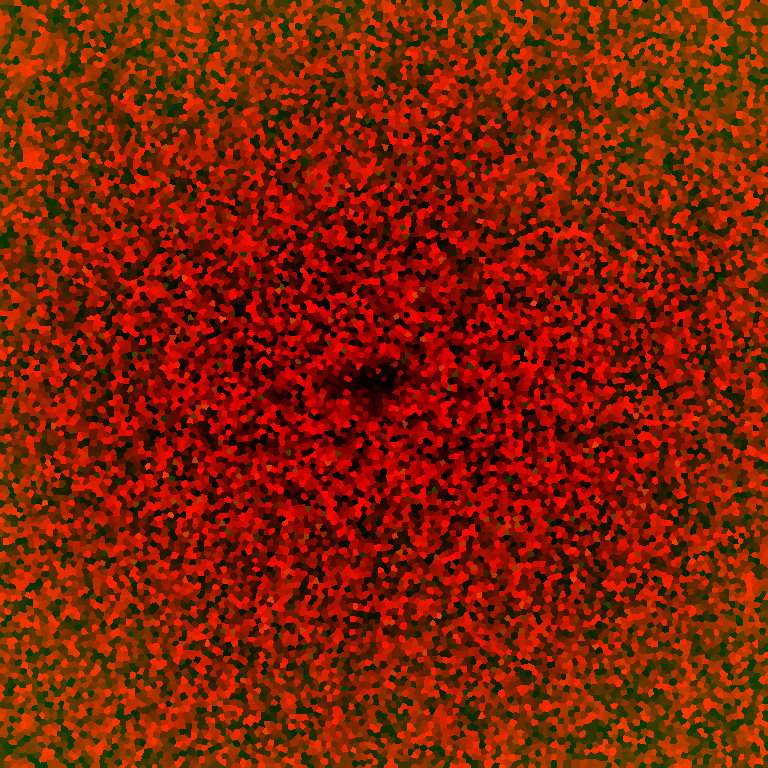
}Note that I use all three colors of the FBO to encode a higher accuracy for the height-map, which gives it a freaky appearance when displaying directly:
The actual heightmap evolution can be seen below.
Results
Note: The visualizations for this project were made using my homemade TinyEngine. The code that I used for height-map meshing and lighting can be found [here].
The system produces nice topographical diversity, showing a number of key features:
- Strong fault lines forming at divergent boundaries
- There doesn’t exist a “plate-less surface”
- Cooling effects lead to stable formation of denser, lower regions on the surface
- Collision leads to consistent sediment piling / formation of mountains
- Plates convect individually on the surface
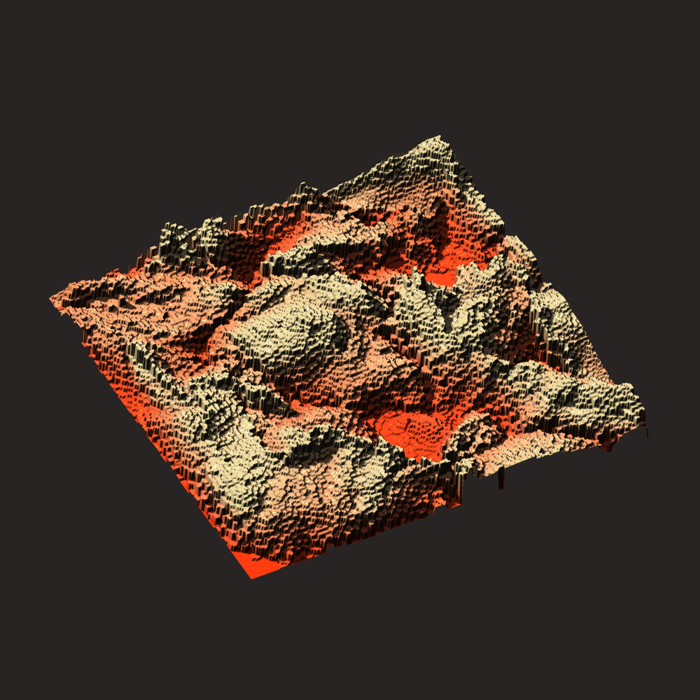
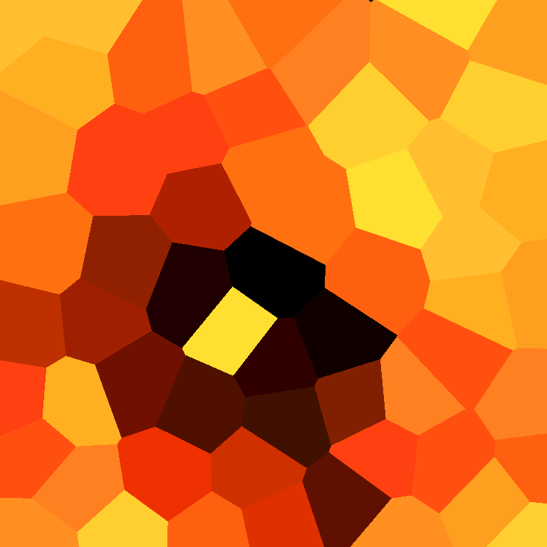
Example images of terrain generated after 1000 cycle steps:
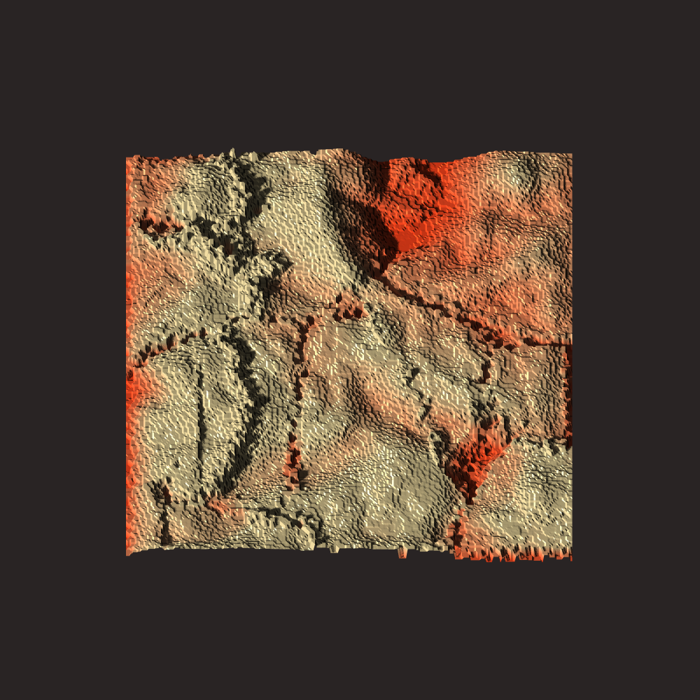
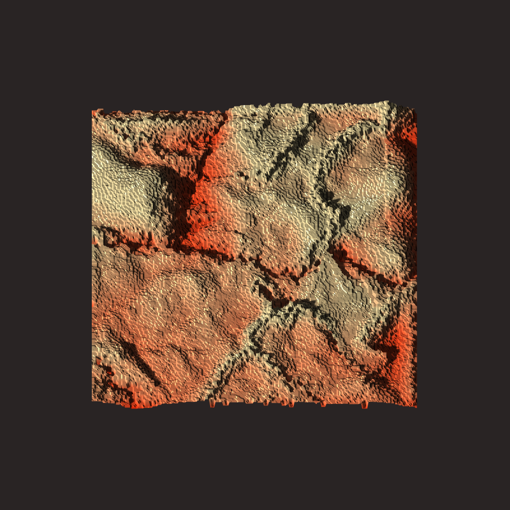
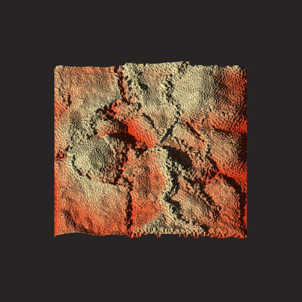
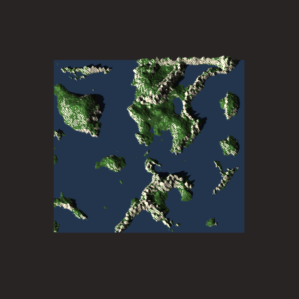
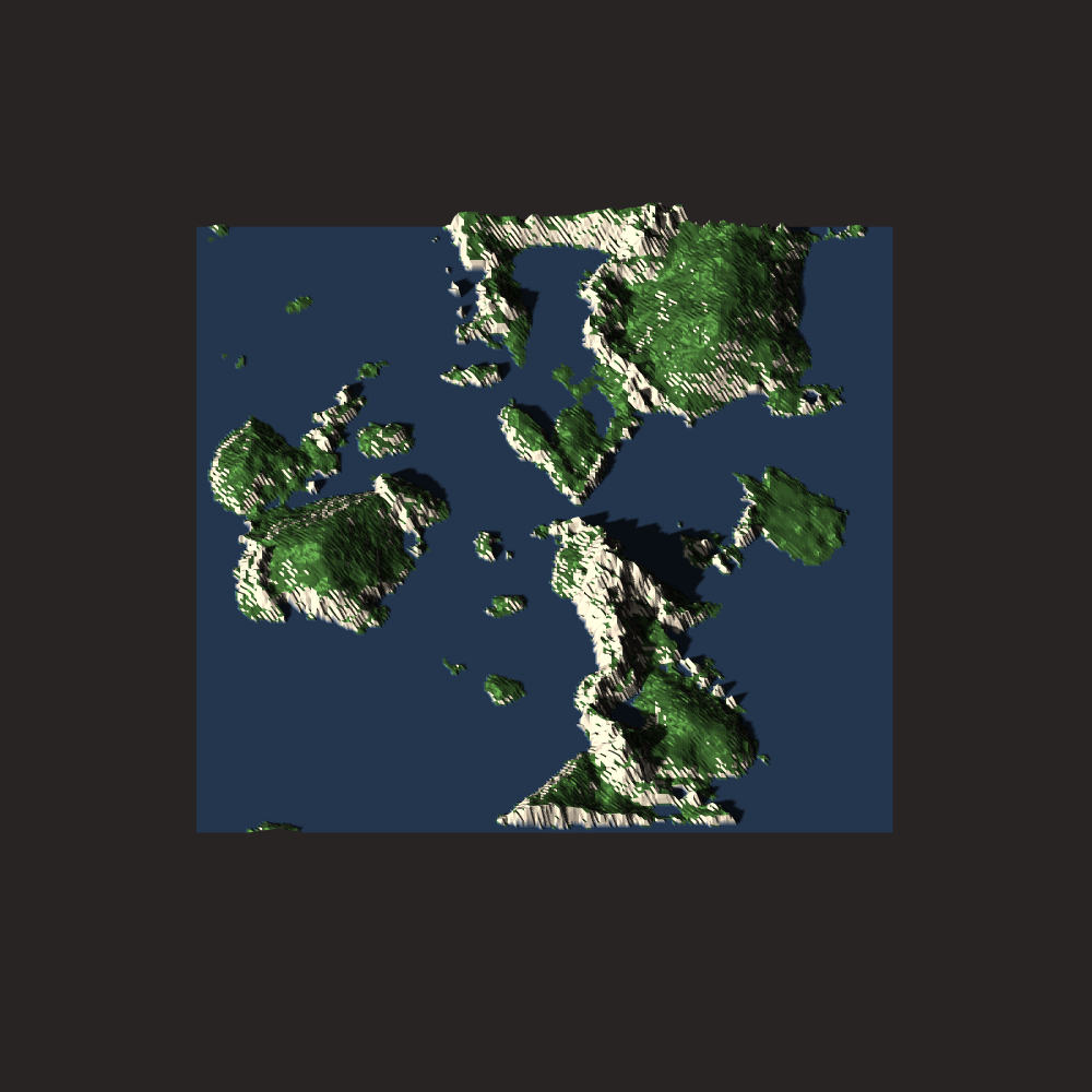
The individual plates have the collective effect of giving the overall topography nice “scarring patterns”.
All videos shown above were real-time, but here is a sped-up version to show the dynamics over longer time-scales :
This produces a hypnotic effect where you can see plates being overrun and melted under less dense plates, while the less dense plates continues to grow at the divergent boundary. The terrain visualization also shows how individual land-masses appear to “move around” the map.
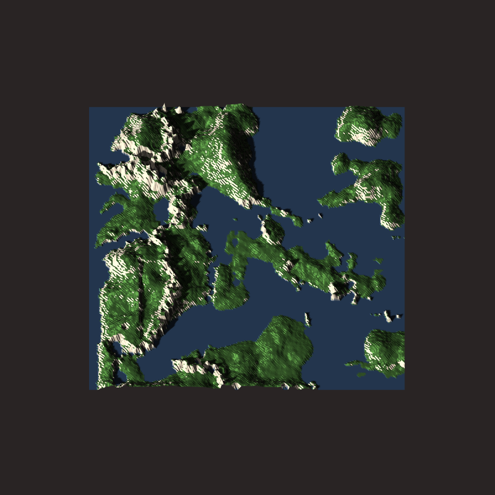
Although the fraction of land area can not be controlled directly, you could simply pick a sea-level to get the fraction of land that you want. Alternatively, you could use the fully sea-less topography and then run a hydrology simulation on it to find the sea-level dynamically.
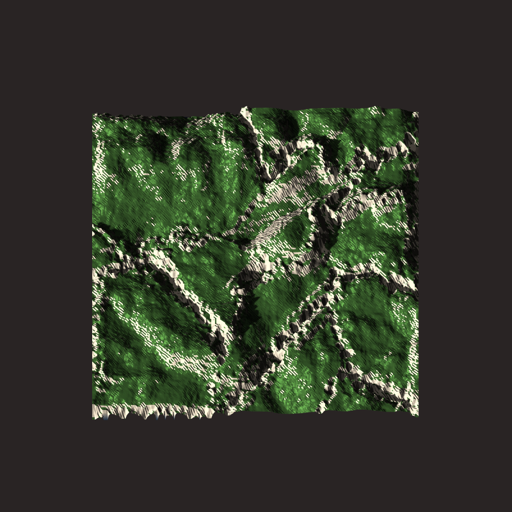
Sea-Level = 0 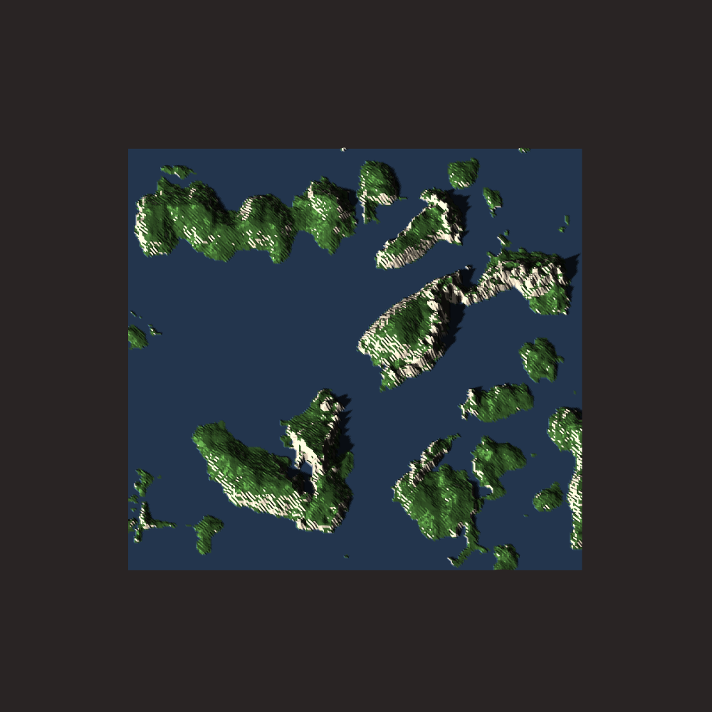
Sea-Level = 0.27 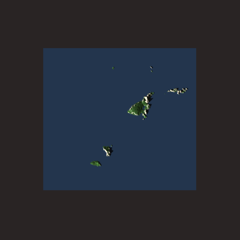
Sea-Level = 0.3 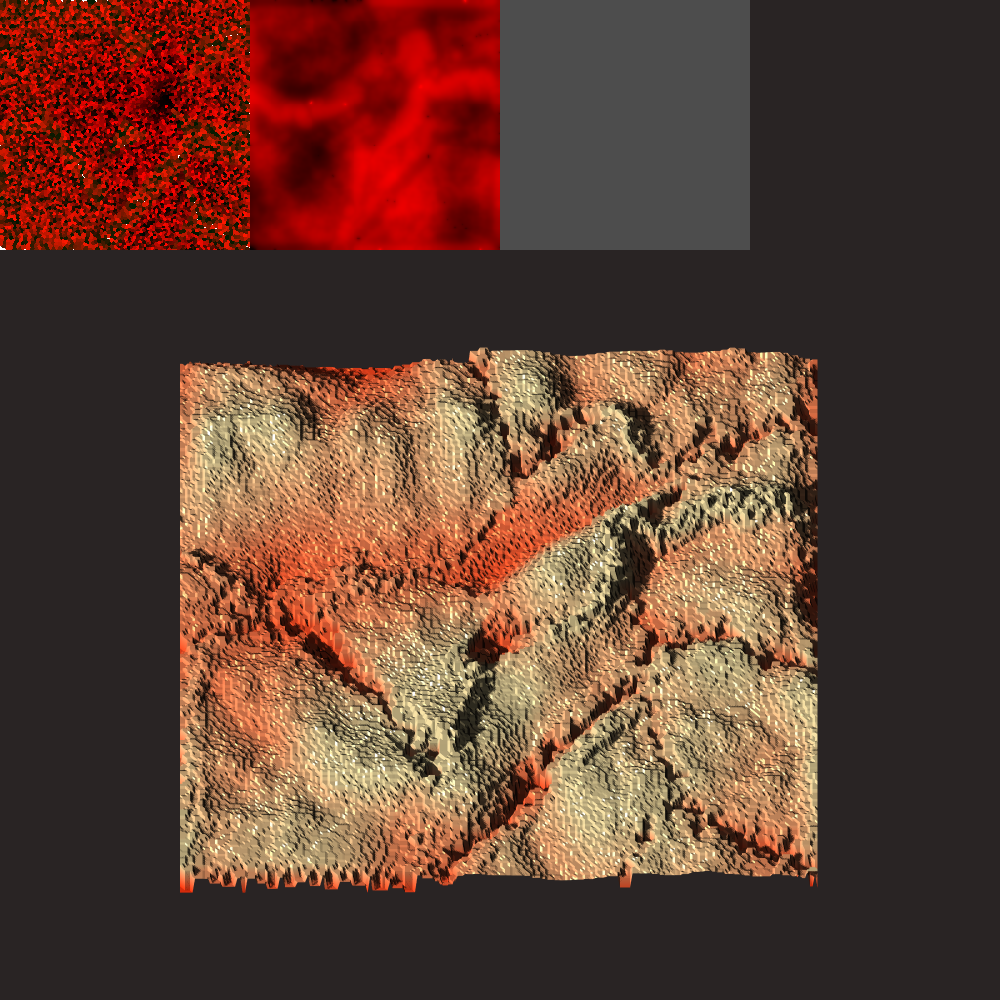
There are some things I am happy about with this system and some aspects which I think warrant improvement.
The clustered convection idea works well and allows to have nice varying properties across the domain while still allowing for a rigid body motion description.
The crystallization description is extremely simple and also works well because it is applied individually at the centroids. The segment interaction at plate boundaries also has some weak concepts of mass-conservation included.
The fact that most of this is implemented in shaders makes it very fast, and allows for fast “area-of-effect” dynamics (e.g. the heating and cooling of the heat-map).
Using a better point-cloud sampler which includes neighboring point information would allow for much easier collision detection and height propagation at collision boundaries. Currently, this process not efficient or elegant. Fast neighborhood information could improve this a lot.
Including erosion cycles between geological plate cycles is not trivially implementable here because the height-map is computed at every step directly from the segment heights. What would be possible is to apply erosion once after a sufficient number of geological cycles has been completed. In that sense, the plate tectonics simulation would only provide an initial terrain and would not be fully coupled.
The physical model could be improved by incorporating a more detailed crystallization process and a more detailed convection model, but I am not sure how to go about this. Including gravitational effects would be interesting but would require more work.
One of my main issues currently is in handling the square boundary. Some clear artifacts can be seen in a number of simulations. This can potentially be mitigated by using a periodic boundary condition. This would also have to be implemented if this system were to be extended to a cube-map for use on a sphere.
I currently also don’t fracture existing plates, although this can be trivially implemented. You can choose a fracture line and spawn two new plate centroids on each side reassigning the original plate’s segments to the new centroids.
The question is: How do you choose where to split plates? Probably some rule with low thickness / density and strong convective forces.
Final Words
The clustered convection system is trivially extendable to a sphere by applying the voronoi texture shader to cubemaps.
Other possible applications of a clustered convection type system could be for 2.5D clouds, weather patterns, water / wave patterns or smoke / fire movement. This would be more for artistic effects though.
In general I want to build a better, more scalable blue-noise sampler that includes neighborhood information. This would be generally useful, but also directly applicable here.
A more rigorous analysis of the applicability of clustered convection to “conservative” systems would also be interesting but would require boundary and neighborhood information.
Additionally, a number of algorithmic optimizations should be possible which would reduce the code-size and probably improve speed by modifying the instanced voronoi render.
Side-Note: More specifically, it should be possible to combine the segments and points into a single struct and avoid a lot of reassignment iteration. This requires utilizing a specific stride when uploading an array of the segment derived class struct to the GPU for the instanced render… blablabla. I could do this but it would require some big modifications to TinyEngine.
One major next step towards a unified terrain generation system would be to design a data-structure for performing height-map operations on a layered structure. This is something I would like to tackle in the near future.
If you have any questions about this system, feel free to contact me!