Simulating Wind on Procedural Terrain using GPU Accelerated Lattice Boltzmann Method

Note: The full source code for this article can be found here (summarized version). Individual sections contain references to specific code snippets below.

For a long time I have been working on generating terrain by simulating geomorphological processes. This primarily includes various forms of erosion, i.e. hydraulic, thermal and wind erosion processes. I believe that in order to generate interesting terrain, you have to simulate processes which are often as complex as they are subtle.

I have always been intrigued by the fact that the atmosphere is a major driving force behind geomorphological processes.

From climatological patterns, to wind-shadow effects and the coupling to vegetation and erosion, the movement of mass and energy through wind is an important contributor.

Initially, I was motivated by the idea of simulating cloud patterns with realistic coupling to the terrain. While highly complex, it always seemed like a fascinating goal.

While I made some previous attempts at simulating clouds, climate and wind patterns, these were all in 2.5D, which I found insufficient to simulate a real micro-climate.

Note: Many interesting atmospheric phenomena, such as updrafts, require a 3D or layered atmospheric model. Some of my previous attempts at atmosphere simulation included Finite Volume Methods and Cellular Automata.

I decided to overcome this by stepping into 3D simulation of wind on terrain using the Lattice Boltzmann Method. I chose to focus on wind simulation first, because a good wind model can act as the base for future atmospheric simulation.

In this article, I want to give context to the relation between the physical and mathematical modelling of fluid flow problems and explain the Lattice Boltzmann Method.

Then I will show how I apply this method to wind on terrain, and present an implementation (with code samples) in GPU accelerated form using compute shaders in OpenGL4 / C++.

Real-Time Wind on Terrain Visualization. The terrain was generated using my SimpleHydrology system (code, article).

Wind as a Fluid Flow Problem

Note: This section assumes familiarity with calculus of integrals and derivatives, in order to relate mathematical and physical models. Feel free to skip it if you are familiar with computational fluid dynamics or are only interested in the implementation.

What is a Fluid?

While we know intuitively that water is a fluid, it surprised me to learn in my first fluid mechanics lecture that the definition of a fluid has nothing to do with gaseous or liquid states of matter. In fact the definition is much more precise.

So what is a fluid?

According to Wikipedia, a fluid is a medium which cannot resist any shear stress applied to it. This means that it does not resist deformation by an external force.

In contrast, a solid resists “deformation” (e.g. by generating an elastic restoring force proportional to the shear force), while a fluid does not and simply deforms.

Note: In general, different types of medium (fluid, solid, viscoelastic fluid, non-newtonian etc.) can be classified by the relation between applied shear-force and internal rate of deformation (a.k.a. “strain”)!

By this definition, air is a fluid, since it behaves like a fluid as defined by its deformation behavior, and thus we can apply the laws of fluid mechanics to it.

Discrete and Continuous Mechanics

While Classical Mechanics models how discrete particles with mass behave under the application of different forces, Continuum Mechanics applies the same principles to a mass where properties change continuously in space.

One well-known result from classical mechanics is the elastic collision (remember physics class?), which results from the application of the conservation of mass, momentum and energy to discrete, colliding masses.

A GPU implementation of N-Ball elastic collisions with boundary conditions. Note that each particle has discrete properties, such as velocity. Applying a constant right-ward body force to all particles gives the appearance of flow around the cylinders. NParticles = 20’000. Source Code

Similarly, a well-known result from fluid mechanics are the Navier-Stokes Equations, which fundamentally encode the principles of conservation of mass, momentum and energy (“conservation laws“); as applied to a continuum.

A similar simulation, where flow around cylinders is shown. Note that we compute a continuous velocity field over the entire domain, instead of at specific locations. This is implemented as a 2D Lattice Boltzmann simulation on the GPU. Source Code

Note: The Navier-Stokes Equations (for newtonian fluids) are derived by combining the differential forms of the conservation laws with a linear relationship for the shear-stress strain relationship, proportional to the fluid viscosity.

The mathematical tool we use to express conservation laws “continuously” are partial differential equations (PDE).

Note: Fluid mechanics is a discipline of continuum mechanics. Continuum mechanics also apply to solid mechanics. The Navier-Stokes equations are partial differential equations.

The (Differential) Conservation Law

A partial differential equation relates the partial derivatives of an unknown multivariable function to each other, thereby describing its behavior in various dimensions (commonly space, time) and implicitly defining the function.

A PDE can be interpreted as a constraint, and solving a PDE means finding functions which satisfy the constraint.

Note: A function which satisfies a given PDE is generally not known, and is generally not guaranteed to exist or be unique, e.g. a PDE can be satisfied by a family of functions.

A differential conservation law is a PDE which describes the behavior of a continuous function of a conserved quantity. We construct the differential conservation law in such a way that it enforces conservation as a constraint (see below).

Writing any physically conserved quantity as a function of time and space, this function must satisfy the differential conservation law PDE constraint in order to be conserved.

How can we express a conservation law as a PDE?

Note: There are different types of PDE, and conservation laws are typically “hyperbolic“. This implies that disturbances in time and space move with finite speed. The other types of PDE are elliptic and parabolic, and exhibit different properties.

The Advection-Diffusion Equation

One of the most basic differential conservation laws is the “Advection-Diffusion Equation“, which describes how mass is conserved for a diffusing, dilute solute in a moving fluid.

(1) $\begin{equation*} \frac{\partial c }{\partial t} = \nabla \cdot (D\nabla c) - \nabla \cdot ( v c ) + R \end{equation*}$

This states that the derivative of the solute concentration in time (at a fixed location) is given by the sum of three terms: The diffusion term, the advection term and the source term.

Note: The diffusion term derives from Fick’s Law, which states that solute flux is proportional to the concentration gradient. The advective flux is proportional to the concentration times the fluid velocity. Taking the gradient of the flux then yields the accumulation, equivalent to (what goes in) – (what goes out). The source term R is the only “non-conservative” term, and describes the generation or destruction of c in the volume.

Setting the source R to 0 means that the only way for mass to enter or leave a volume is by diffusion or advecting across the differential volume boundary, thus conserving mass.

More generally, conservation laws express the constraint:

what goes in minus what goes out is what accumulates inside

For mass, this means mass is never generated anywhere, but has to come from across the boundary (i.e. somewhere else).

Example of the Advection-Diffusion-Equation acting on a 2D function. As the PDE evolves the function time, the integral of the function (i.e. mass / volume) is conserved. Source: Shiyu Ji, Wikimedia Commons

Numerical Solution of PDEs

Given a PDE and sufficient boundary and initial conditions (BC, IC), we wish to find a function which satisfies the PDE.

Integrating PDEs analytically, and in particular the Navier-Stokes Equations, is typically only possible for a small number of well-known problem statements with simple boundary and initial conditions (e.g. Hagen-Poiseuille-Flow).

Solving problems with more complex initial- and boundary- conditions requires making approximations in the form of numerical methods.

Even with numerical methods, solution of PDEs for various problem statements defies a one-size-fits-all approach.

This has spawned a large ecosystem of methods and tools for the solution of PDEs, but most of them involve some form of discretization and subsequent numerical integration of the continuous equations. Each method makes different assumptions and approximations, resulting in varying efficiency, accuracy and stability.

Computational Fluid Dynamics (CFD) therefore concerns itself with the numerical solution of fluid flow problems, and a large area of research is focused on improving the speed, accuracy and stability of these methods for solving PDEs.

One such method is the Lattice-Boltzmann Method. While the Boltzmann Equation is generally more difficult to solve analytically, it has computational advantages as we will see.

Note: The three most common “direct” solution methods for the NSE are the Finite Difference (FD), Finite Volume (FV) and Finite Element (FE) methods. Each uses a different approach to discretising, integrating and boundary condition handling.

– FD: Approximates continuum through point values, approximates derivatives through finite-differences.
– FV: Approximates continuum through cell averages
– FE: Approximates continuum as weighted sum of based functions for interpolating values

A number of more exotic methods exist which solve fluid flow problems not by modelling the continuum directly but by modelling e.g. particles (SPH) or velocity distributions (LBM) in such a way to still fulfil the underlying constraints of the NSE. Both of these methods are more suitable to multi-phase flow.

The Lattice Boltzmann Method

Note: The main source for the following description is the book “The Lattice Boltzmann Method, Principles and Practice” (2017) by Timm Krueger. I recommend reading it for details.

The Lattice Boltzmann Method (LBM) is a numerical method for fluid flow simulation, which similar to other methods aims to satisfy the fundamental conservation laws.

The key difference is that the Lattice Boltzmann Method does not solve for the macroscopic properties of the fluid (density, energy, momentum) directly, but uses a different variable (the Particle Distribution Function) and differential conservation law PDE (the Boltzmann Equation), which together indirectly satisfy the conservation constraints.

Computationally, this change of problem framing represents a new trade-off between parallelism vs. memory efficiency of the problem, which lends itself to GPU acceleration.

In the following chapter, I will present the Boltzmann Equation, its variable the Particle Distribution Function, and how these two concepts relate to our differential conservation laws.

Finally, I will show how the Boltzmann Equation is solved numerically on a lattice as the LBM, and how we can exploit the parallelism of LBM for efficient GPU acceleration.

The Particle Distribution Function

While the Navier-Stokes Equations (NSE) explicitly model the evolution of macroscopic properties (density, energy, momentum) through partial differential equations (PDE), the Boltzmann-Equation is a single PDE which models the evolution of the particle distribution function f, from which these macroscopic properties can be derived.

The particle distribution function f is a probability density, which gives the probability of finding a particle with position x and velocity v at time t.

(2) $\begin{equation*} f(x,v,t) \end{equation*}$

In 2D and 3D, the particle distribution function is a function of 5 and 7 parameters respectively.

Note: One can therefore say that the LBM models the evolution and interaction of a group of particles as described by f.

Deriving Macroscopic Properties

The particle distribution function allows us to derive the original, locally conserved macroscopic fluid properties. In fact, the macroscopic fluid properties can be derived as the moments of the particle distribution function.

The macroscopic density is given by the zeroth moment of f in v, defined as the integral of f over the space of velocities:

(3) $\begin{equation*} \rho(x,t) = \int f\,dv \end{equation*}$

Similarly, the macroscopic momentum density is given by the first order moment of f in v:

(4) $\begin{equation*} \rho(x,t)u(x,t) = \int vf\,dv \end{equation*}$

and the macroscopic total energy density is given by the second order moment of f in v, expressed as:

(5) $\begin{equation*} \rho(x,t)E(x,t) = \frac{1}{2}\int |v|^2f\,dv \end{equation*}$

Note: The quantities shown here are macroscopic densities. Dividing by the density (i.e. zeroth moment or distribution cardinality), gives us our normalized macroscopic quantities.

For a given particle distribution function over space, time and velocity we can thus compute the following quantities:

macroscopic density
macroscopic momentum (from 1)
macroscopic total energy (from 1)
macroscopic bulk velocity (from 1, 2)
macroscopic internal energy (from 4)
temperature, pressure (from 5)

Note: The macroscopic total energy density includes contributions from the internal energy and bulk motion. We isolate the internal energy by computing the second moment with the relative velocity (i.e. subtract the bulk velocity).

The Boltzmann Equation

The Boltzmann-Equation is a partial differential equation which describes the evolution of the particle distribution function f. Taking the total derivative of f wrt. time we get:

$\begin{equation*} \frac{df}{dt} = \bigg(\frac{\partial f}{\partial t}\bigg)\frac{dt}{dt} + \bigg(\frac{\partial f}{\partial x_\beta}\bigg)\frac{dx_\beta}{dt} + \bigg(\frac{\partial f}{\partial v_\beta}\bigg)\frac{dv_\beta}{dt} \end{equation*}$

which can be simplified to the Boltzmann Equation:

$\begin{equation*} \frac{df}{dt} = \frac{\partial f}{\partial t} + v_\beta \frac{\partial f}{\partial x_\beta} + \frac{F_\beta}{\rho}\frac{\partial f}{\partial v_\beta} = \Omega(f) \end{equation*}$

by expressing the change of position as proportional to velocity and change of velocity as proportional to force.

Note: The total derivative of a function wrt. to its arguments captures all contributing terms to the change of a quantity.

This resembles a differential conservation law similar to the advection-diffusion equation. The first two terms relate the change of the distribution at a position due to advection of the distribution with velocity v. The third term represents changes in the distribution due to some force F.

Finally, the entire equation is equal to a source term Ω, which represents the redistribution of f in time due to particle collisions, and is thus known as the collision operator.

Choosing the collision operator such that the conservation law constraints are fulfilled is what allows the Boltzmann-Equation to model the macroscopic behavior of a fluid and thus the Navier-Stokes Equations.

Note: The Boltzmann-Equation provides a second order accurate approximation of the Navier-Stokes Equations. For a detailed derivation on how and to what accuracy the Boltzmann-Equation approximates the NSE, I refer you to the book “The Lattice Boltzmann Method – Principles and Practice” by Tim Krüger or Chapman-Enskog theory.

The Collision Operator

A valid collision operator should enforce the conservation of mass, momentum and energy as well as the relaxation of the distribution to equilibrium. How do we enforce this?

We know that the collision operator Ω is equal to the total derivative of our particle distribution function f:

$\begin{equation*} \frac{df}{dt} = \Omega(f) \end{equation*}$

Using the fact that the total derivative of our conserved macroscopic quantities is zero (by definition), we can apply the expressions for these quantities as the moments of f to directly enforce the conservation constraints on Ω.

For mass conservation, we can write:

$\begin{equation*} \frac{d\rho}{dt} = \frac{d}{dt}\int f\,dv = \int \frac{df}{dt}\,dv = \int \Omega\,dv = 0 \end{equation*}$

and similarly for momentum and energy conservation:

$\begin{equation*} \int v\,\Omega\,dv = 0 \end{equation*}$

$\begin{equation*} \int |v|^2\,\Omega\,dv = 0 \end{equation*}$

respectively.

A valid collision operator must satisfy these constraints!

The simplest collision operator which satisfies the stated constraints is the BGK collision operator, named after Bhatnagar, Gross and Krook. Others include the two-relaxation-time or multi-relaxation time operators.

The BGK Collision Operator

The BGK collision operator explicitly forces the relaxation of the distribution towards its equilibrium distribution:

$\begin{equation*} \Omega(f) = \frac{1}{\tau}(f - f_{eq}) \end{equation*}$

where tau represents the relaxation time.

Finally, the equilibrium distribution is given by the well-known Maxwell-Boltzmann Distribution, which describes the speeds of particles for an idealised gas, given by:

$\begin{equation*} f_{eq} = \rho\bigg(\frac{1}{2\pi RT}\bigg)^{3/2}e^{-|v|^2/(2RT)} \end{equation*}$

The choice of relaxation time and time-step results in the kinematic viscosity being given by:

$\begin{equation*} \nu = c_s^2(\tau - \frac{\Delta t}{2}) \end{equation*}$

where cs is the speed of sound.

Note: It appears that the relation between our choice of collision operator with the relaxation time and the definition of our equilibrium distribution constrains the kinematic viscosity to this expression, which can be derived via Chapman-Enskog Theory. I’m sorry for not deriving the equilibrium distribution for you, but I am sure you can find more qualified explanations!

The Lattice Boltzmann Equation

“Solving” the Boltzmann-Equation means finding a function f which satisfies this differential relation for our collision operator Ω and appropriate initial and boundary conditions.

To solve the Boltzmann-Equation numerically, we need to discretize the particle distribution function in its arguments: space, time and in particular velocity, and finally integrate.

The resulting equation is the Lattice-Boltzmann-Equation.

We can utilize the common method of having discrete time-steps on a lattice / grid for our space and time discretization. Discretizing velocity space is a unique feature of the Lattice-Boltzmann method, and is described below.

Discretizing Velocity Space

Instead of modeling a distribution f of particles over all possible velocities in 2D or 3D, we choose a discrete set of “base velocities” v_i and assume that all particles in the system can only move with one of these velocities.

With this assumption, we can rewrite f as a distribution in time and space for each individual velocity component:

(6) $\begin{equation*} f(x,v_i,t) = f_i(x,t) \end{equation*}$

A natural choice of velocity set is a set of velocities where after one time-step dt, a particle moves exactly to the position of a neighboring lattice element.

Thus the velocity set is fully defined by choice of “neighborhood” and dimension of the problem. In LBM, the velocity sets are therefore commonly named DdQq, where d is the dimension of space and q is the size of neighborhood.

This discretization of the velocity space is what is most commonly associated with the Lattice-Boltzmann method and yields the iconic “velocity set distribution” graphics.

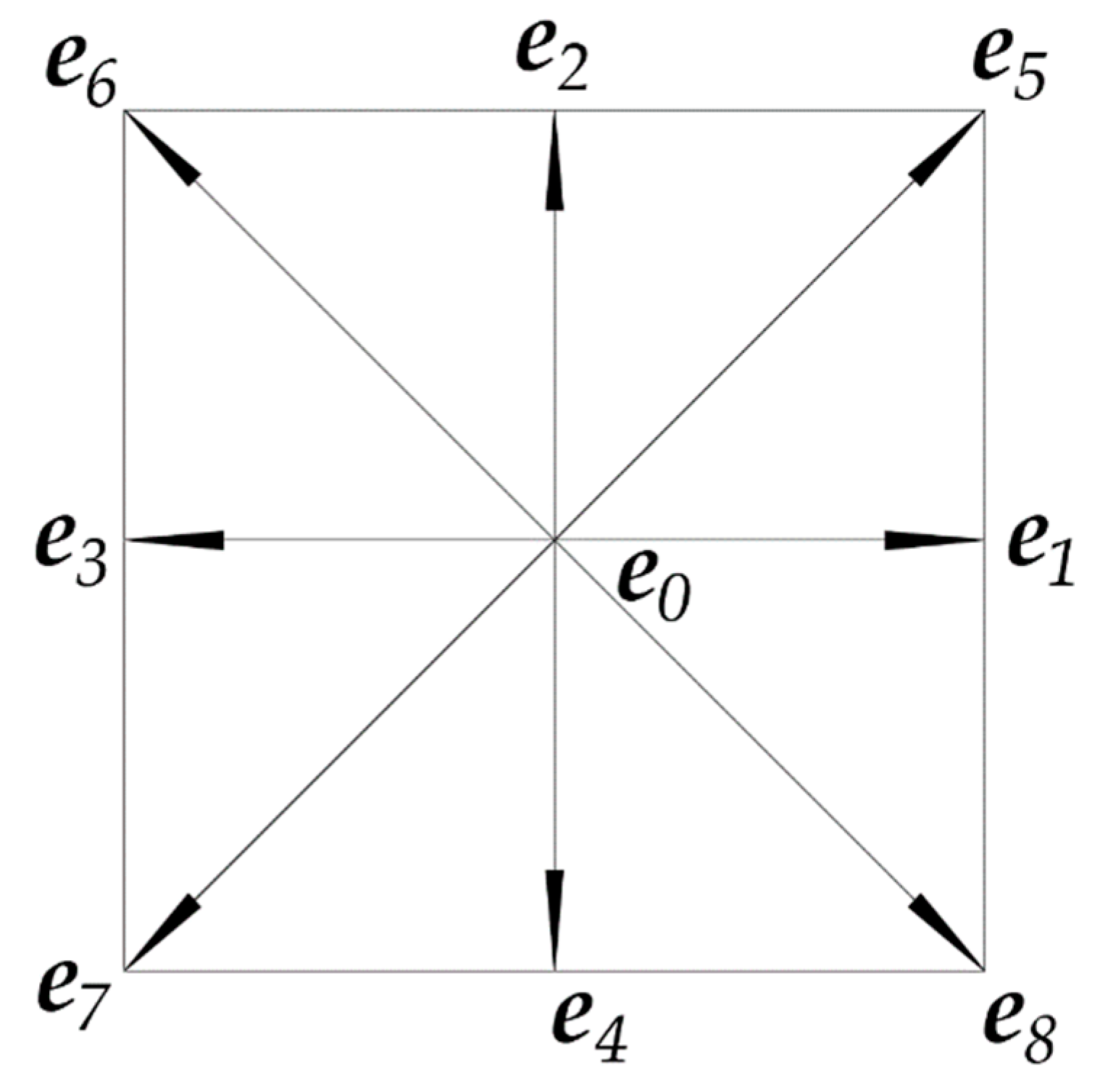
Energies | Free Full-Text | Study on Flow and Heat Transfer Characteristics of Porous Media in Engine Particulate Filters Based on Lattice Boltzmann Method | HTML — The D2Q9 LBM unit velocity set.

For 2D problems, a common choice is the D2Q9 velocity set, while for 3D problems a common choice is the D3Q19 set. Note that the zero-velocity is also a component of the set.

In practical terms, the velocity discretization means:

We must store an array of values of f at every position in space x_i, for every element of the velocity set v_i at every time-step t_i.

This is why the LBM is associated with a larger memory footprint than direct macroscopic property solvers.

Deriving Macroscopic Properties

Using our newly discretized velocity space, the integral expressions for our macroscopic properties as moments of the particle distribution function simplify to summations:

(7) $\begin{equation*} \rho(x,t) = \sum_if_i(x,t) \end{equation*}$

(8) $\begin{equation*} \rho(x,t)u(x,t) = \sum_iv_if_i(x,t) \end{equation*}$

Note: In an implementation, f_i is strictly only defined at discrete time-steps and lattice locations.

Solving the Lattice-Boltzmann Equation

To solve the Lattice-Boltzmann Equation, we can discretize the Boltzmann-Equation in space, time and velocity space:

$\begin{equation*} f_i(x + v_i \Delta t, t + \Delta t) = f_i(x, t) + \Omega_i(x,t) \end{equation*}$

where our new discretized collision operator is given by:

$\begin{equation*} \Omega_i(x,t) = - \frac{f_i - f_i^{eq}}{\tau}\Delta t \end{equation*}$

and our new discretized equilibrium distribution is given by:

$\begin{equation*} f_i^{eq}(x,t) = w_i\rho\bigg(1+\frac{uv_i}{c_s^2}+\frac{(uv_i)^2}{2c_s^4}+\frac{u^2}{2c_s^2}\bigg) \end{equation*}$

Solving this equation sequentially in time is very straightforward!

We can iteratively compute the next time-step using the so-called collision and streaming steps.

Note: While the Lattice-Boltzmann Equation has a larger memory footprint, it is easy to solve and parallelize because it is a hyperbolic differential equation, which is easy to time-step and which only depends on local values.

The Collision Step

The collision (or relaxation step) is an intermediary step which consists of computing the distribution function after collisions, but before particles have moved:

$\begin{equation*} f_i^{*}(x,t) = f_i(x,t) - \frac{\Delta t}{\tau}(f_i(x,t) - f_i^{eq}(x,t)) \end{equation*}$

The Streaming Step

The streaming step consists of moving our intermediate values to their next locations on the lattice. This can either be by “pushing” or “pulling” depending on implementation:

$\begin{equation*} f_i(x + v_i\Delta t,t + \Delta t) = f_i^{*}(x,t) \end{equation*}$

Boundary Conditions

Finally, to conclude our theoretical background on the Lattice-Boltzmann Method, we will take a look at how we can introduce basic boundary conditions into a simulation.

Note: For our situation, we will only consider straight boundary conditions which align with the borders between lattice nodes.

Boundary conditions for the LBM are not applied to the macroscopic properties, but are instead applied to the population distribution function f.

The simplest “link-wise” boundary condition is the so-called bounce-back (BB) boundary condition. The idea is that when a particle meets a rigid boundary, it is reflected back to its original location with its velocity reversed.

$\begin{equation*} f_\hat{i}(x_B,t + \Delta t) = f_i^{*}(x_B,t) \end{equation*}$

where the hat notation ^ refers to the reverse direction:

$\begin{equation*} v_\hat{i} = -v_i \end{equation*}$

and the B subscript refers to any node with at least one boundary connecting to a “solid” node.

The BB boundary condition effectively implements a stable macroscopic no-slip boundary condition for a resting wall. It also guarantees strict mass conservation and is very straightforward to implement.
**Source:** The Lattice Boltzmann Method, Principles and Practice by Tim Krueger, Modified Visualization

Note: An alternative commonly used boundary condition are the so-called wet-node schemes, which instead explicitly define the populations f at the boundary nodes. The key difference is that link-wise schemes consider the boundary to be between nodes, while the wet-node schemes considers the boundary to be on the nodes.

GPU Accelerated Implementation

The key steps to solve the Lattice-Boltzmann Equation are:

Define the lattice and the velocity set
Define the initial and boundary conditions
Compute the local macroscopic fluid properties
Perform the collision step
Perform the streaming step
Apply the boundary conditions and any forces
Start next time-step from step 3

This algorithm was implemented in C++ with TinyEngine as the base for implementing the GPU acceleration code. The provided implementation uses OpenGL4 compute shaders operating on shader storage buffer objects (SSBOs).

The entire code is implemented using 4 compute shaders: lbm.cs, init.cs, collide.cs, stream.cs, with lbm.cs acting as an “include” shader for shared definitions. In the following section, I will detail implementations for both 2D and 3D.

Memory Layout and Allocation

After defining the size of our domain (i.e. NX, NY and NZ), we choose a velocity set depending on the dimensionality. A common choice for 2D is D2Q9, and a common choice for 3D is D3Q19. This defines the full GPU memory footprint.

Our main GPU storage buffers are the particle distribution function array, a propagation array, macroscopic quantities which we store for efficiency and our boundary condition.

Note that for every lattice node in our domain, we have 1 value for each macroscopic property, but Q values of the particle distribution function (one for each velocity comp.).

The particle distribution function and propagation buffers therefore have size N^d*Q, while the macroscopic quantities and boundary conditions have size N^d.

For our implementation, we simply declare our buffers with the correct size on the CPU. Note that we index these buffers with a flattened index in the shader code.

//main.cpp
// Initialize our Arrays (NX*NY*Q)

Buffer f(NX*NY*Q, (float*)NULL);      //Raw F Buffer
Buffer fprop(NX*NY*Q, (float*)NULL);  //Raw FProp Buffer

// Computed Quantities (For Efficiency, NX*NY)

Buffer rho(NX*NY, (float*)NULL);
Buffer v(NX*NY, (glm::vec4*)NULL);

// Boundary Condition (NX*NY)

Buffer b(NX*NY, (float*)NULL);        //Boundary Condition

We then bind these buffers as SSBOs to our main shaders:

// main.cpp
// Initialization Compute Shader

Compute init("shader/init.cs", {"f", "fprop", "b", "rho", "v"});
init.bind<float>("f", &f);
init.bind<float>("fprop", &fprop);
init.bind<float>("b", &b);
init.bind<float>("rho", &rho);
init.bind<glm::vec4>("v", &dirbuf);

// Collision and Streaming Compute Shaders

Compute collide("shader/collide.cs", {"f", "fprop", "b", "rho", "v"});
collide.bind<float>("f", &f);
collide.bind<float>("fprop", &fprop);
collide.bind<float>("b", &b);
collide.bind<float>("rho", &rho);
collide.bind<glm::vec4>("v", &dirbuf);

Compute stream("shader/stream.cs", {"f", "fprop", "b"});
stream.bind<float>("f", &f);
stream.bind<float>("fprop", &fprop);
stream.bind<float>("b", &b);

Note: Because of the GLSL std430 storage layout specifier specification, the velocity vector has to be bound bound as a vector of vec4 in the 3D case.

and access them in the shader using:

//lbm.cs
// Main Buffers and Parameters

layout (std430, binding = 0) buffer f {
  float F[];
};

layout (std430, binding = 1) buffer fprop {
  float FPROP[];
};

layout (std430, binding = 2) buffer b {
  float B[];
};

//init.cs, collide.cs
#version 460 core

layout(local_size_x = 16, local_size_y = 1, local_size_z = 16) in;

#include lbm.cs

layout (std430, binding = 3) buffer rho {
  float RHO[];
};

layout (std430, binding = 4) buffer v {
  vec4 V[];
};

//stream.cs
#version 460 core

layout(local_size_x = 16, local_size_y = 1, local_size_z = 16) in;

#include lbm.cs

layout (std430, binding = 3) buffer rho {
  float RHO[];
};

Note: Not every shader needs access to every buffer.

2D and 3D Velocity Sets

It is convenient to define our velocity set, directions and weights in a small shader code for use throughout in lbm.cs.

D2Q9 Velocity Set Shader Code

//lbm.cs
// 2D LBM

uniform int NX = 256;
uniform int NY = 128;
const int Q = 9;

// Velocity Set

// Weights
const float w[Q] = {4.0/9.0, 1.0/9.0, 1.0/9.0, 1.0/9.0, 1.0/9.0, 1.0/36.0, 1.0/36.0, 1.0/36.0, 1.0/36.0};

// Complementary Direction Index
const int cp[Q] = {0, 3, 4, 1, 2, 7, 8, 5, 6};

// Directions
const ivec2 c[Q] = {
  ivec2(0, 0),
  ivec2(1, 0),
  ivec2(0, 1),
  ivec2(-1, 0),
  ivec2(0, -1),
  ivec2(1, 1),
  ivec2(-1, 1),
  ivec2(-1, -1),
  ivec2(1, -1)
};

D3Q19 Velocity Set Shader Code

//lbm.cs
// 3D LBM

uniform int NX = 64;
uniform int NY = 64;
uniform int NZ = 64;
const int Q = 19;

const float w[Q] = {
  1.0/3.0,
  1.0/18.0, 1.0/18.0, 1.0/18.0, 1.0/18.0, 1.0/18.0, 1.0/18.0,
  1.0/36.0, 1.0/36.0, 1.0/36.0, 1.0/36.0, 1.0/36.0, 1.0/36.0,
  1.0/36.0, 1.0/36.0, 1.0/36.0, 1.0/36.0, 1.0/36.0, 1.0/36.0
};

const ivec3 c[Q] = {
  ivec3( 0,  0,  0),
  ivec3( 1,  0,  0), ivec3(-1,  0,  0),
  ivec3( 0,  1,  0), ivec3( 0, -1,  0),
  ivec3( 0,  0,  1), ivec3( 0,  0, -1),
  ivec3( 1,  1,  0), ivec3(-1, -1,  0),
  ivec3( 1,  0,  1), ivec3(-1,  0, -1),
  ivec3( 0,  1,  1), ivec3( 0, -1, -1),
  ivec3( 1, -1,  0), ivec3(-1,  1,  0),
  ivec3( 1,  0, -1), ivec3(-1,  0,  1),
  ivec3( 0,  1, -1), ivec3( 0, -1,  1)
};

const int cp[Q] = {
  0,
  2, 1, 4, 3, 6, 5,
  8, 7, 10, 9, 12, 11,
  14, 13, 16, 15, 18, 17
};

Equilibrium and Macroscopic Quantities

Using our velocity set, we can define an equilibrium function and functions to compute the macroscopic velocities and densities for a given lattice node.

//lbm.cs
const float cs = 1.0/sqrt(3.0);
const float cs2 = 1.0/cs/cs;
const float cs4 = 1.0/cs/cs/cs/cs;

// Parameters

const vec2 init_velocity = vec2(0.0, 0);
const float init_density = 1.0;

// Compute the Equilibrium Boltzmann Distribution

float equilibrium(int q, float rho, vec2 v){

  float eq = w[q]*rho;
  eq += w[q]*rho*(dot(v, c[q]))*cs2;
  eq += w[q]*rho*(dot(v, c[q])*dot(v, c[q]))*0.5*cs4;
  eq -= w[q]*rho*(dot(v, v))*0.5*cs2;
  return eq;

}

// Compute the Density at a Position

float getRho(uint ind){
  float rho = 0.0;
  for(int q = 0; q < 9; q++)
    rho += F[q*NX*NY + ind];
  return rho;
}

// Compute the Momentum at a Position

vec2 getV(uint ind){

  vec2 v = vec2(0);
  for(int q = 0; q < 9; q++)
    v += F[q*NX*NY + ind]*c[q];
  return v;

}

The Collision Step

The collision step begins by computing our macroscopic density and velocity and storing these values in their respective buffers. It then writes the propagated values / post collision values of the particle distribution function to fprop for each node using the BGK collision operator.

//collision.cs
const float tau = 0.6;
const float dt = 1.0;

void main(){

  const uint ind = gl_GlobalInvocationID.x*NY + gl_GlobalInvocationID.y;

  // Macroscopic Quantities

  const float _rho = getRho(ind);
  const vec2 _v = getV(ind)/_rho;

  RHO[ind] = _rho;
  V[ind] = _v;

  // BGK Method: Compute next Distribution Values!

  for(int q = 0; q < Q; q++){
    FPROP[q*NX*NY + ind] = (1.0 - dt/tau)*F[q*NX*NY + ind] + dt/tau*equilibrium(q, _rho, _v);
  }

}

The Streaming Step

The streaming step subsequently checks the boundary condition, bounces back if it encounters a wall, and otherwise uses a push scheme to propagate the particle distribution function values along their velocity direction.

//stream.cs
void main(){

  const uint ind = gl_GlobalInvocationID.x*NY + gl_GlobalInvocationID.y;

  for(int q = 0; q < Q; q++){

    // Stream-To Position (Push Scheme)

    ivec2 n = ivec2(gl_GlobalInvocationID.xy) + c[q];
    if(n.x < 0 || n.x >= NX) continue;
    if(n.y < 0 || n.y >= NY) continue;

    const int nind = n.x*NY + n.y;

    // Bounce-Back or Push

    if(B[nind] == 0.0)
      F[q*NX*NY+nind] = FPROP[q*NX*NY+ind];
    else
      F[cp[q]*NX*NY+ind] = FPROP[q*NX*NY+ind];

  }

 
}

Initial and Force Boundary Conditions

We can use this equilibrium distribution function to initialize our particle distribution function directly in a shader init.cs. This shader is dispatched once at the beginning.

//init.cs
#version 460 core

layout(local_size_x = 32, local_size_y = 32) in;

#include lbm.cs

void main(){

  uint ind = gl_GlobalInvocationID.x*NY + gl_GlobalInvocationID.y;

  // Initialize the Boltzmann Distribution

  for(int q = 0; q < Q; q++)
    F[q*NX*NY + ind] = equilibrium(q, init_density, init_velocity);

}

Additionally, a Dirichlet-style force boundary condition can be imposed by setting the particle distribution function as equal to the equilibrium distribution that satisfies the BC.

//stream.cs 
// Optional: Force Boundary Condition

  vec2 force = 0.2f*vec2(1, 0);

  if(
    gl_GlobalInvocationID.x == 0
  ||  gl_GlobalInvocationID.x == NX-1
  ||  gl_GlobalInvocationID.y == 0
  ||  gl_GlobalInvocationID.y == NY-1
  )
    for(int q = 0; q < Q; q++)
      F[q*NX*NY + ind] = equilibrium(q, 1.0, force);

Results

With proper initialization and alternating between collision and streaming steps, our computed and stored macroscopic quantities can be used by other shaders directly to generate visualizations of the fluid simulation in real time.

2D Lattice Boltzmann Method

The first test I implemented to check the implementation is to check if vortex shedding occurs in 2D. Here, I am visualizing the x and y components of the velocity as RG.

The implementation successfully worked for more complex and arbitrary boundary conditions.

We can also visualize the flow’s vorticity using a shader-based implementation of the curl operator:

Note: The artefacts on the boundary are a result of the method of computing the curl, which requires accessing neighbouring values. This fails at the boundary.

3D Lattice-Boltzmann Method

In the 2D version, an image is a natural choice for visualizing the macroscopic properties. Visualizing the 3D method is less straight forward.

I found an acceptable method to be using short streamlines, which can visualize velocity by their direction and length.

Here is a visualization of flow around a sphere, with the streamlines colored using their velocity vectors, and transparency added to streamlines with a direction close to the equilibrium velocity.

Take care when implementing streamlines to make sure that vertex positions are updated correctly. If you update each vertex position for every streamline at each time-step, then your streamline is only valid for a static velocity field.

Once your velocity field changes, the entire streamline has to be recomputed to be consistent with the velocity field.

Note: This is because for a given line x_i at time-step t_0, we know that x_1 = x_0 + dt*v(x_0) and x_2 = x_1 + dt*v(x_1). If we move x_0 to x_1 and x_1 to x_2, then at time-step t_1 we won’t have x_2 = x_1 + dt*v(x_1) because the velocity changed.

Therefore, I found that the best method for implementing streamlines was using geometry shaders. A particle swarm can move through the velocity field, each spawning a stream line generated from the velocity field at each time step.

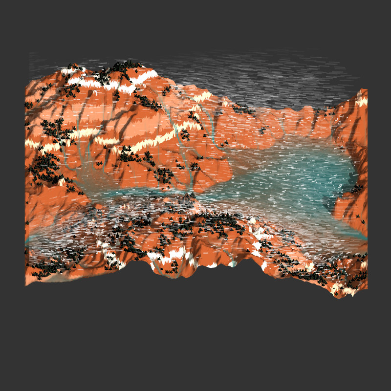
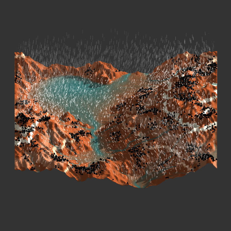
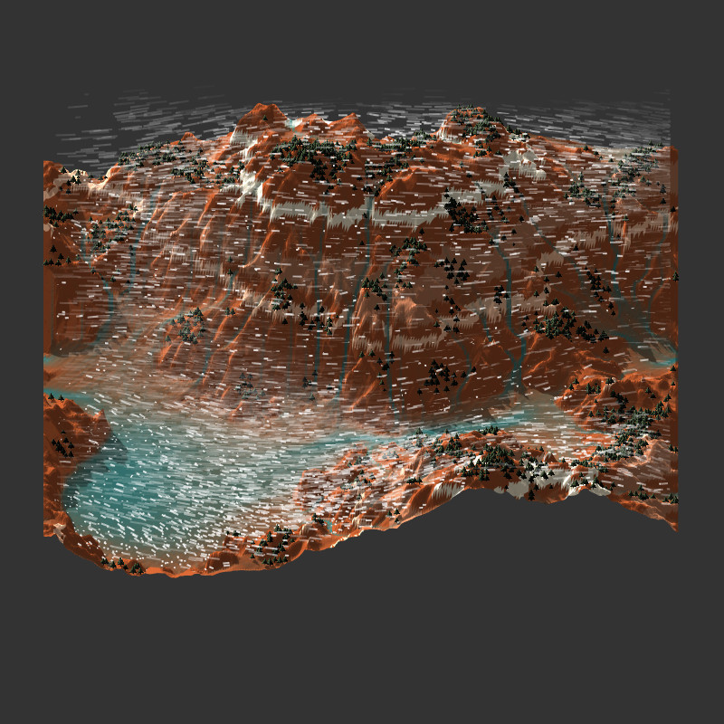
Terrain as Boundary Condition

Finally, implementing terrain as a boundary condition is as simple as generating a heightmap with your tool of choice, and then determining which lattice nodes are considered boundary nodes and which ones aren’t.

This creates very nice visualizations in 3D:

Note: This video was sped up 4x because otherwise the video file would be too large.

Here is the same method implemented on top of SoilMachine, my unified geomorphology simulator. This video is sped up 4x as well.

A video of wind blowing over dunes in real time, simulated in SoilMachine.

With the availability of the surface normals of the terrain, in theory it would be possible to incorporate a more complex boundary condition which doesn’t discretely “voxelize” the terrain (e.g. a wet-node boundary condition or a distributive bounce-back boundary condition). This is beyond the scope of this article though.

Final Words

It took me a very long time to publish this article, because I was very distracted in the last months with real life, and writing it alone took a lot of time. I tried to take care and provide a sufficiently detailed theoretical background into why the Lattice Boltzmann Method simulates fluids. Still, I am glad that it is finally out and that others can see the code!

One aspect which I struggled with while developing this system was controlling the trade-off between accuracy, speed and stability of the simulation without affecting the effective viscosity of the fluid. I believe that I need to reexamine the dimensionality of the domain and the relation between effective viscosity and simulation parameters to gain better control over this.

There are many other aspects which I would have liked to explore, like transport systems (for moving humidity and temperature), but I couldn’t get sufficient results to make it worthwhile showcasing in this article (which is already long).

In the future, I think it would be interesting to see how the wind simulation can be more tightly coupled to the terrain generation itself. Currently, the wind simulation is a mere one-way coupling, and assumes a static terrain. Ultimately, deriving a dynamic rainfall density map coupled to the terrain would be my goal.

Additionally, performance improvements could have the potential to increase the resolution, which I believe are required for a proper mass / energy transport (i.e. cloud) simulation. I believe that I have pushed my integrated GPU to the limit on this one though.

As always, if you have any questions about the system or the code, feel free to reach out to me.