Deriving Wijmans-Hao Type Transport Correlations for Composite Membranes

In this brief contribution, a theoretical justification is presented for the Wijmans-Hao gas transport correlation [1], which relates the mass-transfer restriction factor in a composite membrane to the porosity / morphology of its support layer and geometric properties of its bulk layer.

The corresponding derivation shows that the correlation corresponds to a two-step transport process.

This simplified transport model offers insight into which assumptions the Wijmans-Hao transport correlation makes (mathematically) with respect to the real system, and how the model can be modified and extended to less ideal and even alternate, partially restricted composite membrane systems with distributed properties.

A corollary result describing the permeance lowering effect of a non-uniform pore distribution is presented at the end.

Introduction

The description of mass-transfer across a membrane with one partially restricted interface is a general problem, with application to e.g. composite membranes with porous support structures or membranes with non-permeable surface deposits.

For composite membranes with a porous support, Wijmans and Hao have successfully simulated this mass-transfer problem using CFD to generate a simple correlation be- tween the restriction factor Ψ and the support layer’s properties. [1] This result is commonly cited for its accuracy, simplicity and ease of application. Related attempts at an analytic description suffer from high complexity or inaccuracy in describing the actual gas transport problem.

The lack of theoretical framework for the correlation offers little insight into how the model can be extended to alternate but related membrane systems, or generalized for distributed interface morphologies.

This represents the main motivation for the derivation of a general theoretical description of the restricted interface membrane mass-transfer problem presented in this work.

The resulting two-step transport model is capable of generating a Wijmans-Hao type transport correlation. It also opens new avenues for extending the transport correlation to alternative interface morphologies, including distributed and unstructured interface morphologies.

Note: Some extension possibilities are described at the end, but a full description is beyond the scope of this contribution.

Transport Problem Description

We wish to describe the mass-transfer across a non-porous membrane, where one interface has a restricted area due to a non-permeable covering. The system (1D, simplified) is shown schematically in Figure 1.

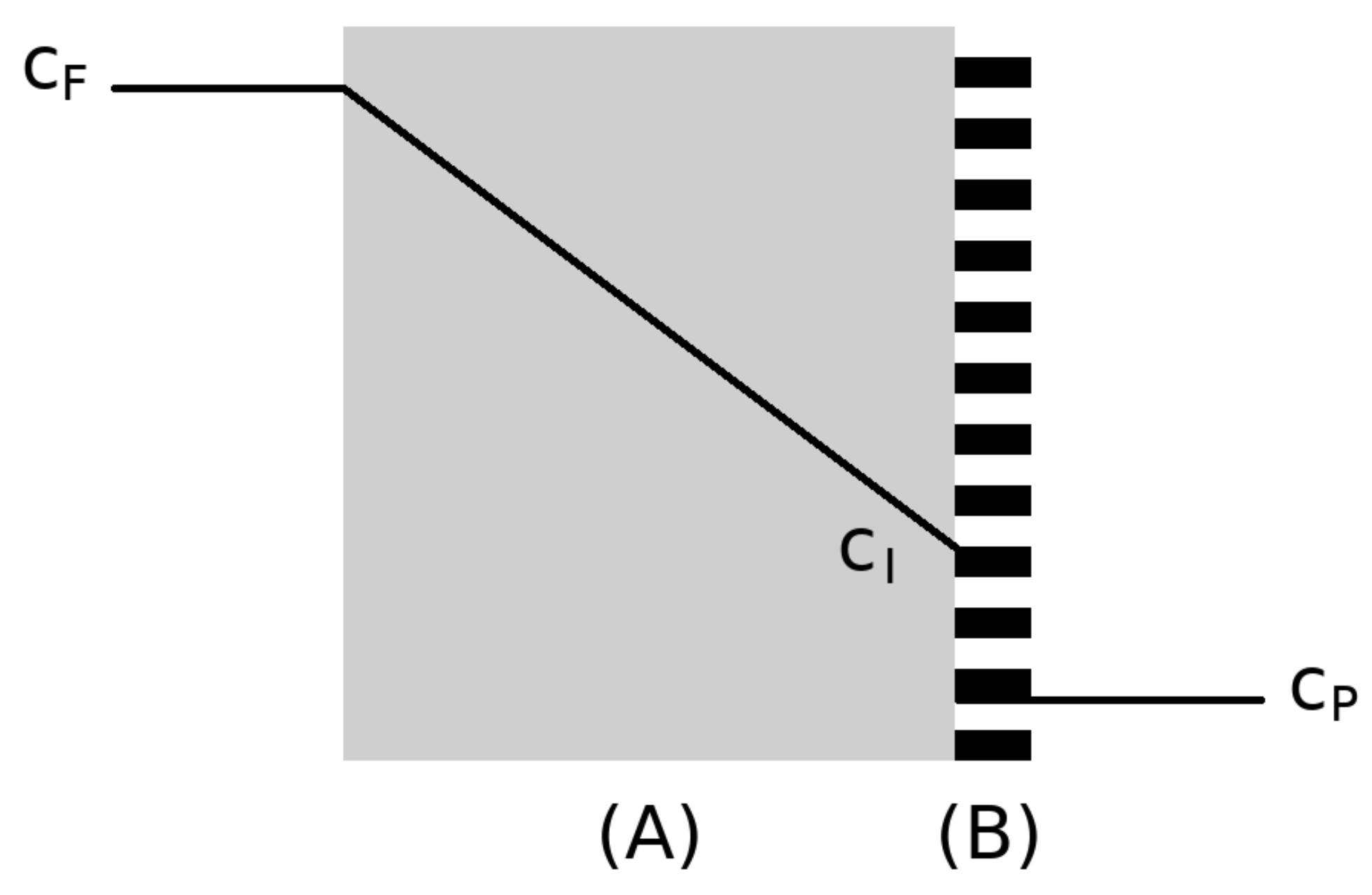
**Figure 1:** 1D-representation of the non-porous membrane (A) and the one-sided restricted interface (B).

The non-restricted fraction of the interface is given by its porosity φ. We assume that the interface has negligible permeability for covered portions, and negligible mass- transfer resistance otherwise.

The gas-flux J across the non-restricted membrane (i.e. φ = 1) is described by the intrinsic mass-transfer coefficient (MTC) k = D/H, where D is the diffusion coefficient and H is the width of the bulk membrane. Thereby, J = k(cF − cP), where cF and cP are the open and restricted interface concentration boundary conditions respectively.

Introduction of the restricted interface (i.e. φ < 1) leads to a relative reduction of the total flux by a ”restriction factor” Ψ ∈ [0, 1):

(1) $\begin{equation*} \Psi = \frac{(D/H)_{eff}}{(D/H)} = \frac{k_{eff}}{k} \end{equation*}$

as described by Wijmans and Hao, and given by the ratio of the effective MTC kEff over the intrinsic MTC k.

Lower mass-transfer results from steeper concentration gradients at the boundary and longer diffusion paths.

In the 1D simplification of this model, the restricted interface represents a discontinuity in the diffusion area at the membrane boundary. The linear steady-state concentration profile thus requires a discontinuity of the interface concentration.

In the real 3D (or 2D) model, we have diffusion through the non-blocked area and equilibriation with the boundary condition cP. At the blocked regions of the interface, we have a higher concentration c > cP, leading to an average interface concentration c̄ I > cP.

This is intuitively visualized in a graphic generated from the simulations of Wijmans and Hao (see Figure 2).

**Figure 2:** 2D visualization of the concentration profile near the restricted interface for a single opening. The concentration is equal to **c_P** at the opening as a boundary condition (blue), while it is larger behind the blocked regions, giving a different average interface concentration.
**Source: Wijmans and Hao [1]**

Using the average interface concentration and equating the steady state fluxes across the system’s components:

(2) $\begin{equation*} J = k\Psi(c_F - c_P) = k(c_F - \bar{c_I}) \end{equation*}$

allows us to re-express the restriction factor:

(3) $\begin{equation*} \Psi = \frac{c_F - \bar{c_I}}{c_F - c_P} = \bigg(\frac{\partial \bar{c}}{\partial x}\bigg)_I \bigg(\frac{H}{\Delta c}\bigg) \end{equation*}$

as given by Wijmans and Hao and valid at steady state.

Summarizing the geometric properties of the system in a hyper-parameter θ. Finding an expression for Ψ(φ,θ) represents the remaining task for describing the mass-transfer across the restricted interface membrane system.

Wijmans-Hao Correlation

The transport problem as described in the previous section was simulated using CFD by Wijmans and Hao to correlate the restriction factor to the porosity and the composite membrane’s geometric properties.

To do this, full mass-transport was simulated with appropriate boundary conditions and the restriction factor was computed using equation 3 from the average concentration gradient at the interface.

The resulting values were then correlated using a function that satisfies the limits:

(4) $\begin{equation*} \lim_{\phi \to 0}\Psi = 0 \end{equation*}$

$\begin{equation*} \lim_{\phi \to 1}\Psi = 1 \end{equation*}$

$\begin{equation*} \lim_{\tau \to 0}\Psi = \phi \end{equation*}$

$\begin{equation*} \lim_{\tau \to \infty}\Psi = 1 \end{equation*}$

where τ = H/R is the ”normalized thickness” and R is the pore radius, resulting in:

(5) $\begin{equation*} \Psi = \frac{\phi + 1.6N_R^{1.1}}{1+1.6N_R^{1.1}} \end{equation*}$

where NR is the ”dimensionless restriction number”:

(6) $\begin{equation*} N_R = \frac{\tau\phi}{1 - \phi} \end{equation*}$

This correlation was computed for a uniform pore grid such that the porosity is given by:

(7) $\begin{equation*} \phi = \frac{\pi R^2}{4L^2} \end{equation*}$

where L is the half-distance between pores.

The accuracy of the correlation was evaluated for non-uniform pore sizes and non-uniform pore distributions, showing good agreement across a wide range of interface geometries.

Two-Step Transport Process

Note: The two-step transport process can be considered a toy model which allows us to analyze under which assumptions the Wijmans-Hao transport correlation approximates a real model.

A relationship between the restriction factor and membrane properties can be derived analytically based on a few assumptions. It is convenient to introduce a dimensionless concentration ξ given by:

(8) $\begin{equation*} \xi = \frac{c - c_P}{c_F - c_P} \end{equation*}$

Note that using Equ. (3), the dimensionless average interface concentration is thereby related to the restriction factor by:

(9) $\begin{equation*} \bar{\xi_I} = 1 - \Psi \end{equation*}$

and the boundary conditions are similarly given by ξF = 1 and ξP = 0. The approach to deriving an analytical expression for Ψ is to find an expression for ξ̄I.

To achieve our goal of finding an expression for ξ̄I, we redefine the transport problem as a two-step process, whereby gas diffuses across the membrane to either an open or a blocked site. For blocked sites, gas then diffuses to a non-blocked site in a subsequent step. This represents the key assumption that simplifies the transport problem for further analysis, and is visualized in Figure 3.

**Figure 3:** Schematic of the two-step diffusion process. Gas that diffuses from the feed (F) to a blocked site (B) must diffuse to the pore exit (P) in a separate step. Relevant MTCs for the various steps and geometric parameters are indicated in the graphic.

We define an additional dimensionless concentration ξ̄B as the average blocked site concentration. We rewrite ξ̄I as:

(10) $\begin{equation*} \bar{\xi}_I = \phi\xi_P + (1-\phi)\bar{\xi}_B = (1-\phi)\bar{\xi}_B \end{equation*}$

Depending on assumptions we make about or interface morphology, we can derive an expression for our steady-state average boundary concentration ξ̄B and express Ψ.

Note: We have not made assumptions about the distribution of blocked sites or how mass is moved between different types of sites. Currently, we just assume their existence.

In the following, I will present a base-case resulting from a series of assumptions about our interface morphology, and show how the Wijmans-Hao transport correlation results.

Locally Averaged Blocked Sites

In the base-case, we assume a blocked site which exists as an averaged site over an area A. We can consider this an average over some local “area of influence”.

Additionally, the locally averaged blocked site is decoupled from the other blocked sites and communicates only with a single, local exit site.

Note: For Wijmans-Hao, the locally averaged blocked site was the periodically repeating grid-cell around a pore.

We express a mass balance over the average blocked site concentration using effective parameters:

(11) $\begin{equation*} \hat{V}_B\frac{\partial \hat{\xi}_B}{\partial t} = \hat{A}_B \hat{k}_B (1-\hat{\xi}_B) - \hat{A}_E \hat{k}_E\hat{\xi}_B \end{equation*}$

where kB represents the average MTC from F to B and kE represents the average “exit” MTC from B to P.

Note: The ^ (hat) indicates that this is given for a specific site.

We also assume a differential volume VB in which ξB is averaged, and effective transport areas AB and AE.

Note: ξB here is an average quantity over an area, and this mass balance is only valid when we define effective kE, kB, AB and AE. Note also that this mass balance is valid for an averaged site, but that there can be multiple averaged sites with different properties.

We express the averaged ξB at steady-state as:

(12) $\begin{equation*} \hat{\xi}_B = \frac{\hat{A}_B \hat{k}_B}{\hat{A}_B \hat{k}_B + \hat{A}_E \hat{k}_E} = \frac{1}{1+\hat{N}_R} \end{equation*}$

where NR is the dimensionless restriction number for the averaged blocked site, generally defined by the ratio:

(13) $\begin{equation*} \hat{N}_R = \frac{\hat{A}_E \hat{k}_E}{\hat{A}_B \hat{k}_B} \end{equation*}$

Note: The restriction number being the ratio between transport away from a blocked site to a pore and transport towards a blocked site offers an intuition for the limits of Ψ.

If (NR → ∞), then gas transported to a blocked site reaches a pore immediately, yielding no effective restriction (Ψ → 1).

If (NR → 0), then gas transported to a blocked site never reaches a pore, such that only the fraction transported directly to a pore ever exits (Ψ → φ).

Effective Average Restriction Number

Choosing our effective flux areas AB, AE as proportional to our blocked and non-blocked areas respectively results in:

(14) $\begin{equation*} \hat{A}_B \propto (1-\hat{\phi})\hat{A} \end{equation*}$

(15) $\begin{equation*} \hat{A}_E \propto \hat{\phi} \hat{A} \end{equation*}$

and choosing the MTC ratio as:

$\begin{equation*} \frac{\hat{k}_E}{\hat{k}_B} = \frac{D}{\hat{H}_E}\frac{H}{D} = \frac{H}{\hat{H}_E} = \hat{\tau} \end{equation*}$

where HE is an effective lateral transport distance to an exit site, results in the well known form of the restriction factor NR for a given averaged blocked site:

$\begin{equation*} \hat{N}_R = \hat{\eta}\frac{\hat{\tau}\hat{\phi}}{1-{\hat{\phi}}} \end{equation*}$

where η represents an unknown proportionality constant.

Note: The assumption for the MTC ratio can be justified by stating that the bulk membrane is isotropic, so lateral diffusion has the same diffusion coefficient D; only the path length varies. Wijmans-Hao chose the effective lateral exit distance / path length as proportional to the pore radius.

Non-Distributed Blocked Sites

Assuming that all “averaged blocked sites” are equal, with a precise definition of the relevant MTCs and related flux areas for a specific interface morphology then allows us to express NR, ξB and Ψ(φ,θ), yielding:

(16) $\begin{equation*} \Psi = 1 - (1 - \phi)\bar{\xi}_B = \frac{\phi + \hat{N}_R}{1 + \hat{N}_R} \end{equation*}$

as uniform averaged blocked sites imply that:

(17) $\begin{equation*} \bar{\xi_B} = \hat{\xi_B} = (1 + \hat{N}_R)^{-1} \end{equation*}$

yielding the well known form of the Wijmans-Hao transport correlation for composite membranes.

Wijmans-Hao Model

The Wijmans-Hao transport correlation can be considered a two-step transport model with a single class of averaged blocked site. The effective lateral transport distance from a blocked site to a pore is assumed as proportional to the pore radius. The effective flux areas from the feed to a blocked site and from the blocked site to a pore are proportional to the blocked and non-blocked areas respectively.

In the work of Wijmans and Hao, a value of η ≈ 1.6 provided the best fit for their simulation series. Note that the derived expression for Ψ does not include an exponential factor as given by Wijmans and Hao.

The Wijmans-Hao transport correlation is generally valid under the previously stated assumptions, even for other non-porous interface morphologies.

One key alternative membrane morphology of interest is that of an ”inverted pore” interface, where portions of the interface are blocked by circular deposits instead of having circular pore openings (see Figure 4).

**Figure 4:** Front view of the partially sealed in- terface. Instead of having porous openings with a distribution of the pore size, we have a distri- bution of solid deposits on the surface restricting mass-transfer.

While ”pore radii” are not well defined for this system, as long as we can define the characteristic lateral diffusion distance and make the assumption that the ratio of effective flux areas is given by the void fraction φ/(1-φ), then this model is suitable.

Generalizing the Model

Using the two-step transport model, a number of intuitive generalizations present themselves by eliminating assumptions about the interface morphology.

A full description for removal of the assumptions is beyond the scope of this contribution, as validation of correctness and practicality would require an extensive simulation study.

Non-Uniform Averaged Blocked Sites: We can still assume a partitioning of the entire interface into locally averaged blocked sites. Instead of a single class of blocked sites, we assume a distribution of blocked sites and use a distribution of restriction numbers NR to express ξ̄B and Ψ.

Effective Average Restriction Number: We can drop assumptions about the functional form of the effective average restriction number. The effective average flux areas do not have to be directly proportional to the blocked and non-blocked areas respectively. The same is true for the effective lateral diffusion distance.

Coupled Blocked Sites: The Wijmans-Hao transport model assumes the existence of averaged blocked sites, which are decoupled from each other and communicate only with a local exit site. An alternative model would be to consider a coupling between multiple blocked and exit sites separately.

Non-Averaged Blocked Sites: Instead of using locally averaged blocked sites as a basis for deriving the average interface concentration, it could be possible to express a mass balance for a point-concentration on the blocked interface and compute the average blocked site concentration directly. The morphological properties of the interface can be fully defined by a signed distance function.

Corollary Results

Permeance Lowering Effect of a Non-Uniform Pore Distribution

Using our expression for the restriction factor as derived by our two-step transport model, we can give a straightforward mathematical justification for the permeance-lowering effect of a non-uniform pore distribution.

We assume that the restriction factor Ψ is a function of the random variable NR, our dimensionless restriction number.

We note that the function Ψ(NR) is concave for all φ ∈ (0, 1) and all η > 0:

(18) $\begin{equation*} \Psi(N_R) = \frac{\phi + \eta N_R}{1 + \eta N_R} \end{equation*}$

According to Jensen’s inequality, the expectation value of the concave function F of a random variable X is smaller than or equal to the function of the expectation value of X:

(19) $\begin{equation*} F(\mathbb{E}[X]) \geq \mathbb{E}[F(X)] \end{equation*}$

We note that for a non-uniform distribution of restriction numbers, the expected restriction factor is E[Ψ(NR)]. For a uniform restriction number distribution, the expected restriction factor is Ψ(E[NR]).

This means that permeance is lower for a non-uniform pore distribution than for a uniform pore distribution, even if they share the same mean restriction number.

Bibliography

[1] Wijmans, J. G., and Pingjiao Hao. “Influence of the porous support on diffusion in composite membranes.” Journal of membrane science 494 (2015): 78-85.