Simple Particle-Based Hydraulic Erosion

Note: The full source code for this project , as well as an explanation on how to use and read it, can be found on Github [here].

I took a break from my Master thesis this week to work on something I have been putting off for a while: Improved terrain generation for my Territory project. Hydraulic erosion is a simple, low effort method for this – so that’s what I did!

This worked really well as a one-day coding challenge and wasn’t as complicated as I expected. The results are fast to generate, have physical meaning and look amazing.

In the following article, I will present my simple C++ implementation of a particle-based hydraulic-erosion system on a square grid. I explain the physical reasoning behind the implementation and present the math. The code is extremely simple (about 20 lines total for erosion math) and fast to implement, so I encourage anyone looking to improve their terrain realism to try it.

The results are rendered using a stripped-down version of my Homebrew OpenGl Engine, which I modified to render a 2D array of points as a height-map. The stripped down version of the engine is much easier to understand if you are interested in learning OpenGL in C++.

Implementation

Inspired by a number of other resources on hydraulic erosion, I decided particle systems made the most sense.

The erosion process using particles is then simple:

Spawn a particle at a random position on the surface
It moves / slides over the surface using normal classical mechanics (explained below)
Perform mass-transfer/ sedimentation between the surface and the particle (explained below)
Evaporate a part of the particle
If the particle is out of bounds or is too small, kill it
Repeat for however many particles you want.

Note: System parameters are explained in the relevant section. The most important is a time-step factor “dt”, which scales all parameters proportionally. This allows you to increase simulation rate (at the cost of noise) without changing the relative parameter scale. Look for it in the code below.

Particles

To do this, I built a simple particle struct that contains all the relevant properties that I need:

struct Particle{
  //Construct particle at position _pos
  Particle(glm::vec2 _pos){ pos = _pos; }

  glm::vec2 pos;
  glm::vec2 speed = glm::vec2(0.0); //Initialize to 0

  float volume = 1.0;   //Total particle volume
  float sediment = 0.0; //Fraction of volume that is sediment!
};

Note: I use GLM for doing vector operations, in case you are unfamiliar with it.

The particle has a position and velocity, which determines how it moves around. Additionally, it has a volume and a fraction of that volume which is sediment.

Movement: Classical Mechanics

The movement of the particle on the surface is simulated using classical mechanics. In short, the position x of the particle is changed by the velocity v which is changed by the acceleration a.

$\begin{equation*} \[ \frac{d\textbf{x}}{dt} = \textbf{v} \] \end{equation*}$

$\begin{equation*} \[ \frac{d\textbf{v}}{dt} = \textbf{a} \] \end{equation*}$

Note: Bold letters indicate that the quantity is a vector.

We also know that force is equal to mass times acceleration:

$\begin{equation*} \[ \textbf{F} = m\textbf{a} \] \end{equation*}$

The particles experience downward acceleration due to gravity, but it sits on the surface making downward acceleration impossible. Instead, the particle experiences force F along the surface proportional to the surface normal.

Therefore, we can say that the acceleration a is proportional to the surface normal vector n divided by the particle mass.

$\begin{equation*} \[ \textbf{a} = \frac{k}{m}\textbf{n} \] \end{equation*}$

where k is a proportionality constant, and m is the particle mass. If the mass is equal to volume times density, we get our full system for particle motion with classical mechanics:

//... particle "drop" was spawned above at random position

glm::ivec2 ipos = drop.pos; //Floored Droplet Initial Position
glm::vec3 n = surfaceNormal(ipos.x, ipos.y);  //Surface Normal

//Accelerate particle using classical mechanics
drop.speed += dt*glm::vec2(n.x, n.z)/(drop.volume*density);
drop.pos   += dt*drop.speed;
drop.speed *= (1.0-dt*friction);  //Friction Factor

//...

Note: The speed is reduced after moving the particle using a friction factor. Note where the time step factor is included here. Particles have intrinsic inertia proportional to the density, due to modeling their movement using acceleration.

Sedimentation Process: Mass Transfer

The sedimentation process physically occurs by transferring sediment from the ground into the particle and back, at whatever position the particle is (“Mass Transfer“).

In chemical engineering, it is typical to describe the transfer of mass (i.e. change of mass / sediment in time) between two phases (here: the ground and the droplet) using mass transfer coefficients.

Mass transfer is proportional to the difference between the concentration c and the equilibrium concentration c_eq:

$\begin{equation*} \[ \frac{dc}{dt} = k(c_{eq} - c) \] \end{equation*}$

where k is the proportionality constant (mass transfer coefficient). This difference between the equilibrium and actual concentration is often referred to as a “driving force”.

If the equilibrium concentration is higher than the current concentration, the particle absorbs sediment. If it is lower, it loses sediment. If they are equal, there is no change.

The mass transfer coefficient can be interpreted in a number of ways:

The rate of transfer between the phases (here: “deposition rate”)
The speed with which the droplet concentration approaches the equilibrium concentration

Defining our equilibrium concentration fully defines our system. Depending on the definition, our system will exhibit different sedimentation dynamics. For my implementation, the equilibrium concentration is higher if we are moving downhill and if we are moving faster and proportional to the particle volume:

//...

//Compute Equilibrium Sediment Content
float c_eq = drop.volume*glm::length(drop.speed)*(heightmap[ipos.x][ipos.y]-heightmap[(int)drop.pos.x][(int)drop.pos.y]);

if(c_eq < 0.0) c_eq = 0.0;

//Compute Capacity Difference ("Driving Force")
float cdiff = c_eq - drop.sediment;

//Perform the Mass Transfer!
drop.sediment += dt*depositionRate*cdiff;
heightmap[ipos.x][ipos.y] -= dt*drop.volume*depositionRate*cdiff;

//...

Note: The change in concentration inside the particle is described fully by the mass-transfer equation. The change in the height-map is additionally multiplied by the particle volume, because we don’t change it proportionally to the concentration but the mass (concentration times volume).

Other Things

The height-map is initialized using randomly seeded layered Perlin-Noise.

At the end of every time step, the particle loses a little mass according to an evaporation rate:

//...

drop.volume *= (1.0-dt*evapRate);

//...

This process is repeated for thousands of particles spawned at random positions and simulated individually (in my case: sequentially on my CPU).

A good set of parameters is included by default in my implementation. The erosion looks very good after about 200k particles.

Results

The final code for the erosion process is about 20 lines of code without comments.

Here is a before-after comparison for 10 samples. The simulation generates very nice ridges on elevations, with sediment depositing on the sides of some ridges, leading to nice plateaus.

Sample of 10 before-after comparisons. The shader I programmed takes two colors as input. I also implemented shadow mapping, distance fog and phong shading to give it a nice appearance.

Here are 10 more (different) samples of just results:

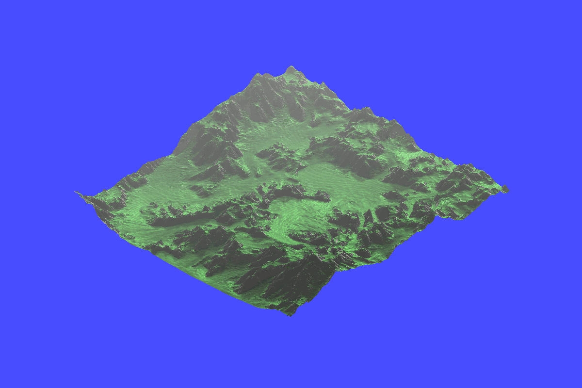
By seeding the initial map differently, it would be possible to produce different results in a directed fashion.

Simulation Time

The simulation time is directly related to the particle lifetime and the number of simulated particles.

Particle lifetime is affected by a number of factors, and can vary significantly on a per-particle basis, because they are spawned at random locations:

Friction and Inertia: How fast do particles move around
Grid-Size: How likely is it that particles fly off the edge
Evaporation Rate: How quickly do particles disappear

With the default parameters, it takes between 10 and 100 microseconds to simulate a single particle, resulting in about 10 to 20 seconds for simulation 200’000 particles.

It is possible to increase the degree of erosion and lower the particle lifetime by increasing the time-step, without changing the number of simulated particles. This can make the simulation more “noisy”, and has the potential to crash the simulation if the time-step is chosen too high.

The actual simulation in the engine has an additional overhead from the re-meshing of the surface for rendering.

Optimizations could include lowering the re-meshing overhead, or increasing the speed of a single time-step for a single particle.

Future Work

I will slap this into my Territory project soon, as the basis for generating the height-map in my terrain generator.

I have already written a simplified fluid dynamics simulation framework for climate systems, but it isn’t ready for publication yet. This system derives climate patterns from a height-map. This will be the subject of a future blog-post for physically accurate procedural climate systems!

Using the simulated climate system, it would be possible to sample the particles from a distribution (i.e. where is the rain?) instead of distributing them uniformly on the map. This would fully couple the terrain geology and the climate, which would be sick.

Additionally, by including different types of geological formations, rocks would have varying degrees of solubility. This would directly affect the mass-transfer coefficient (deposition rate), giving different erosion rates.

This system is not capable of simulating actual fluid flow and rivers, but could potentially be adapted to do so. I will give this some though and maybe follow up in the future.