Note: The code for this article is available on my Github [here].

I spent the entire summer in eastern Pennsylvania near the Delaware river because the MIT campus closed in early March and I had to go home. On the occasional walk to get out of the house / away from my work, I would stroll into the forests, and one day I made a simple observation:

When any branch of a tree splits, the sum of cross-sectional area is conserved.

This observation was apparently already made by Da-Vinci. I decided to use this observation, together with a transport-oriented interpretation of natural tree growth create a simple model and generate some trees.

This article will describe that model and how I use it to generate realistic looking trees with varying morphologies!

Using this technique, you can generate high-quality tree meshes with various stages of growth at runtime with little overhead!

Note: The relevant code for the actual tree growth model can be found in the file “tree.h” and is only about 250 lines of code.

Note: This work was done in April 2020, but I put off writing this article until I completed my thesis project this September.

Growth Model

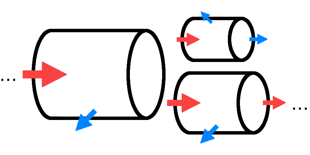
A tree grows by passing nutrients up its branch structure through its outer bark layer. As it does so, each branch segment grows in girth. Nutrients arriving at the end of a non-split branch lead to growth in length, while a split branch passes the nutrients to its child branches proportionally to some ratio. For simplicity, we assume that branches only split in a binary fashion (there exist ternary split plants).

This is shown conceptually in the following image.

We associate each branch with a length and a radius. At every time-step, we have an amount of nutrients entering a given branch. A fraction of the nutrients is consumed and transformed into girth and/or length, and the remainder is passed to the child branches. Finally, if a branch reaches a certain length, it will split and create new child branches.

Fun-Fact: Because a split branch never grows in length, a tire-swing which you hang from an existing branch of a tree will never move its position or height relative to the ground.

Implementation

A binary tree lends itself well to recursive implementation of the growth model, where we handle each branch individually. To do this, we define a branch struct:

struct Branch{

  int ID = 0;         //For Leaf Hashing
  bool leaf = true;   //End of branch?

  Branch *A, *B, *P;  //Child A, B and Parent

  //Growth Parameters
  float ratio, spread, splitsize;
  int depth = 0;

  //Constructors / Destructors

  //No parent
  Branch(float r, float s, float ss):
    ratio       {r},
    spread      {s},
    splitsize   {ss}
  {};

  //With parent
  Branch(Branch* b, bool root):
    ratio       {b->ratio},
    spread      {b->spread},
    splitsize   {b->splitsize}
  {
    if(root) return;
    depth = b->depth+1;
    P = b;  //Set Parent
  };

  ~Branch(){
    if(leaf) return;
    delete(A);
    delete(B);
  }

  //Size / Direction Data
  glm::vec3 dir = glm::vec3(0.0, 1.0, 0.0);
  float length = 0.0, radius = 0.0, area = 0.1;

  //Member Functions
  void grow(double _size);
  void split();

  //Compute Direction to Highest Local Leaf Density
  glm::vec3 leafdensity(int searchdepth);
};

Each branch stores pointers to its parent and child branches. If a branch has no children, the flag “leaf” is set to true. Each branch is also associated with a “depth” on the tree, where the main trunk has depth = 0.

We also store the branch’s geometric information, including its length, radius, area and its direction in space (3D vector).

Finally, the branch struct has two member functions which describe the entire growth process: grow() and split(). These are described in more detail below.

Note: The branch destructor will also destroy all child branches, while child branches are only constructed using the split() method.

Grow

The grow method is very simple to implement. A branch is fed with a fixed amount of nutrients (feed), which is passed to the grow function. This quantity’s dimension can be interpreted as a volume of growth.

void Branch::grow(double feed){

  radius = sqrt(area/PI);   //Current Radius

  //...

If a branch does not have children, we grow its length proportionally to the cube-root of the feed. The feed is then reduced by the consumed amount and the area is grown by the remainder. We finally check if a branch is sufficiently long to split, in which case we split it and return:

  //...

  if(leaf){
    length += cbrt(feed);       //Grow in Length
    feed -= cbrt(feed) * area;  //Reduce Feed
    area += feed/length;        //Grow In Area

    //Split Condition
    if(length > splitsize * exp(-splitdecay * depth))
      split();  //Split Behavior

    return;
  }

  //...

Note: The split condition checks if the length is above a threshold value “splitsize”. In this model, the threshold value decreases as the branch has a higher depth on the tree. The choice of split condition is currently arbitrary and not based on any natural observations.

If the branch is not a leaf, we grow it in girth only and pass a fraction of the feed to its children.

Note that if a branch keeps all the nutrients for itself, it will grow in girth while its child branches will not grow at all. Conversely, if a branch passes all nutrients to its children, the children will grow larger than the original branch.

The pass-ratio thereby also determines whether the sum of cross-sectional area is conserved at a given split in the tree. We can thus exploit the pass-ratio as a degree of freedom to satisfy this constraint in a feedback-control style fashion.

We compute the pass-ratio X from the areas A of all branches at a split point (children A, B and parent P):

   

which is the ratio between the sum of the child branch areas and the total area of all three branches connecting at the split. If the areas of the children are larger than that of the parent, we pass less than half of the feed along (limit X = 0) and the parent branch grows faster. Similarly, if the parent branch area is larger than the sum of children’s areas, we pass more than half of the feed along and the children grow faster (limit X = 1). Therefore, using this definition for the pass-ratio will naturally let the pass ratio approach a value near X = 0.5, implying a conserved cross-sectional area.

Note: X will not approach exactly 0.5 because of how the area growth rate depends on the length of the branch. For a parent branch with children of equal length, X -> 0.5. Not all trees strictly follow this branching rule anyway (see e.g. Baobab tree).

We finally grow the branch accordingly:

  //...

  //Feedback Control for Area Conservation
  double pass = (A->area+B->area)/(A->area+B->area+area);

  area += pass * feed / length;   //Grow in Girth
  feed *= ( 1.0 - pass );         //Reduce Feed

  //...

A species of tree is associated with a parameter that determines how asymmetrically it grows (“ratio”). We pass the nutrients to the child branches according to this ratio:

  //...

  if(feed < 1E-5) return;         //Prevent Over-Branching

  A->grow(feed*ratio);            //Grow Children
  B->grow(feed*(1.0-ratio));
}

and our tree growth model is thus fully described.

Split

The split method is responsible for constructing the child branches (A and B) and attaching them appropriately. We also use the binary tree structure to easily associate each new branch with a unique ID:

void Branch::split(){

  leaf = false;

  //Add Child Branches
  A = new Branch(this, false);
  B = new Branch(this, false);

  //Every Leaf ID is Unique (because binary!)
  A->ID = 2 * ID + 0; 
  B->ID = 2 * ID + 1;

  //...

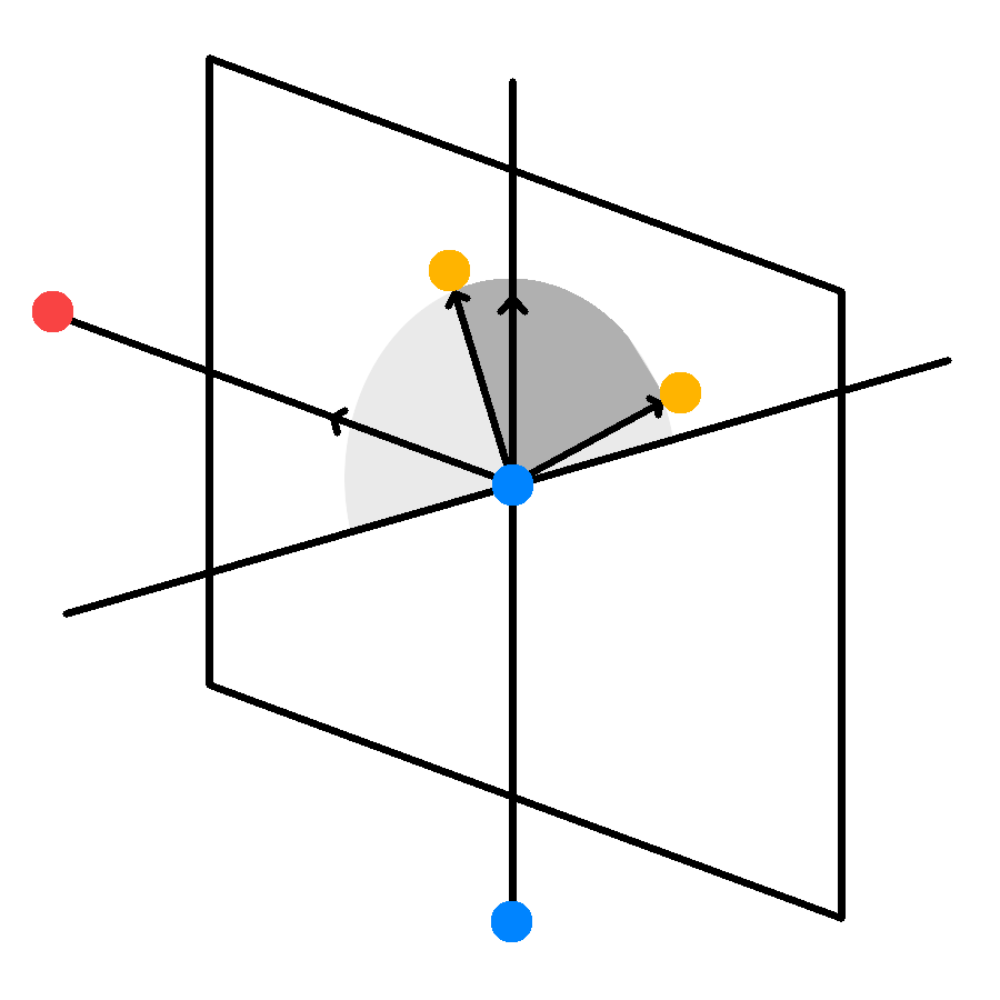
Each child branch then needs to also be given a direction to grow towards. Trees naturally branch out to increase surface area and reduce self shadowing. This is biologically embedded into the genetics of the tree, but we can approximate this behavior by letting the children grow perpendicularly to the plane spanned by the parent branch vector and the vector pointing towards the position with the highest leaf density:

  //...

  /*
  Ideal Growth Direction:
    Perpendicular to direction with highest leaf density! 
  */

  //Direction of Highest Density
  glm::vec3 D = leafdensity(localdepth);    

  //Normal Vector to Plane    
  glm::vec3 N = glm::normalize(glm::cross(dir, D));
  //Reflection
  glm::vec3 M = -1.0f*N;                            

  float flip = (rand()%2)?1.0:-1.0; //Random Direction Flip

  //Mix direction according to split ratio
  A->dir = glm::normalize( glm::mix(flip*spread*N, dir,     ratio) );
  B->dir = glm::normalize( glm::mix(flip*spread*M, dir, 1.0-ratio) );

}

The child branch direction is finally mixed with the direction of the parent branch according to the split ratio, so heavier branches tend to continue straight while light branches will be more perpendicular to the parent branch.

Note: With a random chance, the A branch will be chosen as the heavier branch or the lighter branch. Additionally, a parameter spread can give more weight to perpendicular or straight growth.

The local leaf density is computed with a simple recursive tree search algorithm. We ascend the tree to a certain depth, and then re-descend the tree to compute the average leaf position with lambda function from the geometrical information!

glm::vec3 Branch::leafdensity(int searchdepth){

  //Random Vector! (for noise)
  glm::vec3 r = glm::vec3(rand()%100,rand()%100,rand()%100)/glm::vec3(100)-glm::vec3(0.5);

  //Random vector for trunk
  if(depth == 0) 
    return r;

  Branch* C = this;                               //Ancestor node
  glm::vec3 rel = glm::vec3(0);                   //Relative position to start node
  while(C->depth > 0 && searchdepth-- >= 0){      //Ascend tree
    rel += C->length*C->dir;                      //Add relative position
    C = C->P;                                     //Move to parent
  }

  //Compute Average Leaf Position of all Children (recursive)
  std::function<glm::vec3(Branch*)> leafaverage = [&](Branch* b)->glm::vec3{
    if(b->leaf) return b->length*b->dir;
    return b->length*b->dir + ratio*leafaverage(b->A) + (1.0f-ratio)*leafaverage(b->B);
  };

  //Average relative to ancestor, shifted by rel ( + Noise )
  return directedness*glm::normalize(leafaverage(C) - rel) + (1.0f-directedness)*r;
}

A random noise vector is also mixed in to the direction. The ratio between noise and directed growth can be controlled by the parameter directedness.

Visualization

Note: This tree growth model was visualized using TinyEngine.

The binary tree data structure lends itself well to recursive meshing. Each branch is meshed as a cylinder with a length, radius and taper. The start-point of any branch is given by the end-point of its parent, with its direction defined in the split function. The start point of the root is simply the origin.

// Model Constructing Function for Tree
std::function<void(Model*)> _construct = [&](Model* h){

  //Basically Add Lines for the Tree!
  std::function<void(Branch*, glm::vec3)> addBranch = [&](Branch* b, glm::vec3 p){

    glm::vec3 start = p;
    glm::vec3 end   = p + glm::vec3(b->length*treescale[0])*b->dir;

    //Get Some Normal Vector
    glm::vec3 x = glm::normalize(b->dir + glm::vec3(1.0, 1.0, 1.0));
    glm::vec4 n = glm::vec4(glm::normalize(glm::cross(b->dir, x)), 1.0);

    //Add the Correct Number of Indices
    glm::mat4 r = glm::rotate(glm::mat4(1.0), PI/ringsize, b->dir);

    //Index Buffer
    int _b = h->positions.size()/3;

    //GL TRIANGLES
    for(int i = 0; i < ringsize; i++){
      //Bottom Triangle
      h->indices.push_back(_b+i*2+0);
      h->indices.push_back(_b+(i*2+2)%(2*ringsize));
      h->indices.push_back(_b+i*2+1);
      //Upper Triangle
      h->indices.push_back(_b+(i*2+2)%(2*ringsize));
      h->indices.push_back(_b+(i*2+3)%(2*ringsize));
      h->indices.push_back(_b+i*2+1);
    }

    for(int i = 0; i < ringsize; i++){

      h->positions.push_back(start.x + b->radius*treescale[1]*n.x);
      h->positions.push_back(start.y + b->radius*treescale[1]*n.y);
      h->positions.push_back(start.z + b->radius*treescale[1]*n.z);
      h->normals.push_back(n.x);
      h->normals.push_back(n.y);
      h->normals.push_back(n.z);
      n = r*n;

      h->positions.push_back(end.x + taper*b->radius*treescale[1]*n.x);
      h->positions.push_back(end.y + taper*b->radius*treescale[1]*n.y);
      h->positions.push_back(end.z + taper*b->radius*treescale[1]*n.z);
      h->normals.push_back(n.x);
      h->normals.push_back(n.y);
      h->normals.push_back(n.z);
      n = r*n;

    }

    //No children
    if(b->leaf) return;

    addBranch(b->A, end);
    addBranch(b->B, end);
  };

  //Recursively add Branches (at origin!)
  addBranch(root, glm::vec3(0.0));
};

The growth model is wrapped in a small program which visualizes the tree in color and with shading. A small interface lets you control the growth parameters, visualization and re-grow the tree directly.

Cosmetic leaves were added to the trees using a similar recursion. A particle cloud is spawned at the end-point of any branch which is a leaf branch (past a certain depth). The leaves use the unique ID of each branch to hash the point cloud, so the visualization is steady at every time-step.

Results

In order to grow a tree, we simply construct a branch called “root” and continue to feed it nutrients to let it grow:

int main( int argc, char* args[] ) {

  //...

  Branch* root;
  root = new Branch({0.6, 0.45, 2.5}); //Create Root

  //...

  while(true){ //Not the actual game loop...
    if(!paused)
      root->grow(growthrate);
  }
		
  //...

  return 0;
}

This growth model with the base parameter set produces very realistic looking trees! A small sample of trees of the same “species” is shown below (deciduous):

The parameters which were previously described allow us to alter the tree’s morphology and generate different species. We can tune the split ratio to get trees which grow more asymmetrically, resembling e.g. evergreen trees:

We can also change the tendency with which branches prefer to grow straight or perpendicular, and how strongly they will avoid high leaf-density areas. This leads to a strong resemblance to bonsai-like trees (these look really good!):

The system is thus capable of replicating a wide variety of binary-split branch structures.

Generating trees which resemble specific species is then only a matter of cosmetics and parameters, i.e. choosing specific sprites and colors for the leaf particle clouds and choosing a set of appropriate growth parameters.

Each tree which is generated still contains elements of randomness (specifically during branching), meaning the trees for a given parameter set are similar but unique!

Additional Thoughts

This method allows you to generate high-quality meshes of procedural trees, at various stages of growth and for different morphologies, with very little code / overhead.

Another key advantage of this system is the full tree structure information. The structure is not “baked” into a model, and thus the geometric information can be used in a game context for mechanics such as fruit growth, climbing, destruction, etc.

The constraint of conserved cross-sectional area is imposed here as a boundary condition but does not emerge naturally from a more basic set of assumptions about transport. I was hoping to find an argumentation that was based on nutrient transport restriction but could not express it adequately.

Similarly, past publications claim the the conservation of cross-sectional area is related to structural properties of the tree and its stability and not strictly its transport properties.

The model could be enhanced by considering different types of branches, which spawn other types of branches (similar to an L-system) and have varying parameter sets.

More thought can also be put into how the presence of leaves affects with the growth of the branch structure (nutrient back-transport). For cosmetics, adding an age parameter to each branch would also allow for leaves to “bloom” over time.

A better model for exactly how the growth process occurs in a branch could further enhance the realism, but would probably have a negligible return in terms of visual appeal.